Your Data Science Journey - From Beginning to End

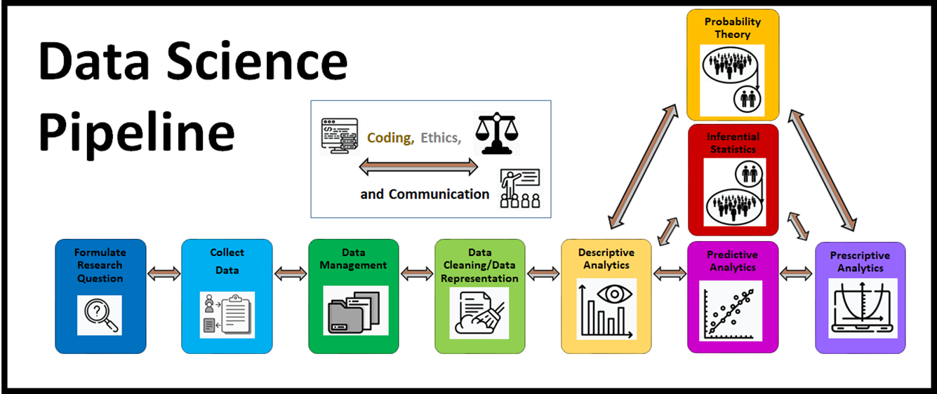
We use the "data science pipeline" to describe many of the common elements a full data science analysis uses. Note that not all of these elements are used in a full data science analysis. Also note that a full data science analysis is not always a linear process, going from left to right. Sometimes, discoveries that we make further on in the pipeline can make us go back to a previous part of the pipeline (like your question that you're trying to answer) and start again to provide a more effective, sensible answer to your original question.

These are considered to be the main elements of the data science pipeline.

1. Formulating a research question and/or goal
2. Collecting the data that can answer this question and/or pursue this goal
3. Data Management – Considering how your dataset will be stored and extracted
4. Data Cleaning/Representation – Considering how/if your data needs to be cleaned or put into a different format for further analysis
5. Descriptive Analytics – Describing your dataset with summary statistics, visualizations, and other sophisticated techniques
6. Predictive Analytics – Using your dataset to make predictions
7. Inferential Statistics – Using your dataset to answer questions about larger populations using a random sample drawn from that population
8. Prescriptive Analytics – Using your dataset to make optimal decisions

Probability Theory is also included, and involves calculating probabilities associated with different outcomes. This tool is used both separately and in combination with inferential statistics and predictive analytics.

Question vs. Dataset

For instance, what you might have discovered in Data Science Discovery is that the type of dataset that we have in our hands can influence the type of research questions that we are able to answer with this dataset.

Question: For instance, which of the following research questions do you think that we can use our Instagram dataset to answer?

1. Is there an association between the number of accounts a particular account follows (number_of_follows) and being/not being a fake account (account_type) in this dataset?
2. Does an account being fake (account_type) make it more likely for the account to follow more people (number_of_follows) in this dataset?
3. Do we have sufficient evidence to suggest that there is an association between the number of accounts a particular account follows (number_of_follows) and being/not being a fake account (account_type) in the population of all Instagram accounts?
4. Do we have sufficient evidence to suggest that an account being fake (account_type) make it more likely for the account to follow more people (number_of_follows) the population of all Instagram accounts?

What you might have noticed is that this dataset was NOT collected using random assignment. That is, we did not randomly assign our Instagram accounts to a treatment (say being fake) and a control (say being real). Therefore, we can NOT answer a research question that implies that some aspect of our explanatory variable (i.e., fake vs. real) causes some effect of our response variable (i.e., number of follows).

Because the phrase "makes it more likely" implies this causal relationship between our explanatory variable and our response variable, we cannot use THIS dataset to answer questions (2) or (4).

However, we can answer question (1)! Evaluating if there is or is not an association between two variables in a dataset that we have in our hands is always something that we can do with the use of summary statistics, visualizations, or more sophisticated descriptive analytics techniques. However, there are actually many ways in which we can try to answer this question and potentially many different answers we could arrive at. We'll look at some examples in the Descriptive Analytics section of how we might do this below.

Also take note that it is POSSIBLE to answer question (3) as well using this dataset that we have in our hands. Take note that question (3) is actually referring to two much larger datasets (i.e., populations) of ALL fake Instagram accounts and ALL real Instagram accounts. However, given that our actual dataset is comprised of two random samples from our two populations of interest, then we can use this dataset to make a valid inference about the nature of our two populations. We'll look at some examples of how we might do this in the Inferential Statistics section below.

Which Comes First?

Given how the nature of our dataset can influence the type of research questions that we can answer with it, full data science analyses usually come in two flavors.

1. Start with a research question/goal that you had in mind first, and then collect and curate the dataset that will help you answer/pursue this specific research question/goal.
2. Start with a dataset that you already have first, and then try to generate interesting questions/goals that you are able to answer/pursue with this dataset.

Effective Communication

Remember, that the typical end of a full data science analysis will involve you trying to effectively communicate the answers to your research questions to your desired audience. Thus, even if you choose to start with a dataset first and answer interesting questions as you go, when composing your final report/presentation, you should state the research questions/goals that you will answer/pursue at the very beginning to help effectively guide the reader through the rest of your report.

Descriptive Analytics

Example

Research Goal:

So suppose that our research goal was to first assess if there is an association account_type and number_of_follows in this dataset (our question (1) above). And then if there is an association, clearly and thoroughly communicate the nature of this association.

The ways that we might go about evaluating whether there exists an association between two variables in a given dataset is going to depend on the types of variables that we're dealing with. Notice that number_of_follows is a numerical variable, while account_type is a categorical variable with two levels (real and fake).

Below we'll showcase three different ways one might try go about pursuing this research goal. Try to think about which one is best. What is it that makes one of these approaches better than the others?

Attempt #1: Comparing Just Two Means

Given that we're dealing with a numerical and a categorical variable, we may decide to calculate the mean number of follows for fake accounts (853.93) and the mean number of follows for real accounts (704.60).

Based off of just these two statistics, we may then make the following hasty, non-robust conclusion.

Conclusion #1: "Because the average number of accounts followed by fake accounts is different from the average number of accounts followed by real accounts, we can claim that there is an association between account_status and number_of_follows in this dataset.
Furthermore, because the mean number of follows for fake accounts (853.93) is GREATER THAN the mean number of follows for real accounts (704.60), we can conclude that fake accounts generally follow MORE people than real accounts in this dataset."

Attempt #2: Comparing Just Two Medians

Why did we call conclusion #1 above not robust? Well let's consider another way that we might try to pursue our same research goal. Again, given that we're dealing with a numerical and a categorical variable, we may decide instead to calculate the median number of follows for fake accounts (163) and the median number of follows for real accounts (470).

Conclusion #2: Because the median number of accounts followed by fake accounts is different from the median number of accounts followed by real accounts, we can claim that there is an association between account_status and number_of_follows in this dataset. Furthermore, because the median number of follows for fake accounts (163) is LESS THAN the median number of follows for real accounts (470), we can conclude that fake accounts generally follow LESS people than real accounts in this dataset.

Attempt #3: More Robust Conclusion Making

Notice how our two conclusions above were saying two different things! So how do we decide which conclusion is more sensible, if at all?

To answer our main research question, we can actually think of our two variables that we're examining in this dataset comprised of two distinct numerical distributions:

• the distribution of the number of accounts followed by fake accounts
• the distribution of the number of accounts followed by real accounts.

Recall that when dealing with a numerical variable, there's actually many more things that we can use to describe this distribution in addition to just measures of center (like the mean and median).

Describing Numerical Distributions

1. Measures of Center
   • Mean
   • Median
2. Measures of Spread
   • Standard Deviation
   • IQR (Interquartile Range)
   • Range
3. Shape
   • Modality
   • Skew
4. Any Outliers

We can use the following side-by-side boxplots visualization below to visualize the median, IQR, a rough sense of skew, and any outliers that belong to these two distributions of follow numbers for fake and real accounts.

Using this plot above gives us a more expansive understanding of the nature of the association of the account_type and the number_of_follows variables in this dataset. By pursuing a more thorough, expansive way of answering this research question, we are more likely to come to a conclusion that is less likely to come at odds with another data scientist's approach to answering this question, provided they too are also attempting to answer this question in a thorough, expansive way.

Conclusion #3:

• Comparing Medians vs. Means

Because at least one of these distributions (the fake accounts) is not symmetric, the mean is not going to be a good way of comparing the measure of centers between the two types of accounts. This is because the median tends to reside towards the center of the distribution (regardless of skew or outliers), while the mean tends to get dragged out in the direction of the skew and/or outliers. Thus, the median provides a more informative summary of the center of both distributions.

• Comparing Medians

Therefore, because the median number of accounts that fake accounts follow (163) is smaller than the median number of accounts that real accounts follow (470), we might be tempted to conclude "fake accounts generally follow less accounts in this dataset".

• Comparing IQR Overlap

However, notice how there is no separation between the two IQR boxes in the two boxplots above. Thus, while the median number of follows for fake accounts is smaller than it is for real accounts, because the middle 50% of observations for both distributions (i.e., the IQRs) overlap so much, this difference of medians is comparatively only very slight when compared to the general spread of the distributions. Thus, "we cannot conclude that there is a strong association between account type and the number_of_follows in this dataset."

However, we can conclude the following:

• The spread of the number of accounts that fake accounts follow is larger.
• From the rough sense of shape visible in the boxplot, it appears that the number of accounts that fake accounts tend to follow might be skewed to the right, while the number of accounts that real accounts follow appears to be more symmetric (with the exception of a few large outliers).
• The median number of accounts that fake accounts follow is smaller than it is for real accounts. However, this difference of medians is small in comparison to the spread of the two distributions.

Why robust answers?

So why is robust research question-answering important?

Because there often exist many competing approaches with which to answer an oftentimes vaguely stated research question, getting in the practice of answering your research questions and pursuing your research goals in as robust a way as possible can have a lot of benefits to both you and society. When we say robust in this context, we mean that your conclusions are more likely to be validated by the approaches and conclusions made by other researchers who are also trying answer the same research question in a robust way.

For instance, two ants looking at different parts of an elephant when faced with the research question "what is this?" may provide two very wrong answers if they approach the question by only looking at the few elements of the elephant right in front of their faces. However, by taking a more expansive, robust approach to answering this question and communicating with each other effectively, the two ants together are more likely to arrive at an answer that is closer to the truth.

Inferential Statistics

Recall how we discussed above that since our dataset is comprised of two random samples of our populations of interest (i.e., ALL fake Instagram accounts and ALL real Instagram accounts), we are able to answer the following research question with this dataset.

Research Question: Do we have sufficient evidence to suggest that there is an association between account_status and number_of_follows for the population of all Instagram accounts?

As with most research questions we might ask, there are many ways that we might attempt to answer this question. And yet again, some of these methods may give us opposing answers!

However, remember ideally we would like for our approach to be robust AND map back onto our main research motivation for asking the question in the first place.

For example, here's two ways in which we might attempt to answer this research question.

A Two Sample t-Test

Setting Up a Hypothesis Test

We can actually use a two-sample t-test to help us answer this question. Specifically, we can use a hypothesis test to test the following null hypothesis and alternative hypothesis given below.

\(H_0: \mu_{fake}=\mu_{real}\)

\(H_A: \mu_{fake}\neq \mu_{real}\)

• \(\mu_{fake}\) is the average number of accounts followed for ALL fake accounts, and
• \(\mu_{real}\) is the average number of accounts followed for ALL real accounts

Implicit Interpretation

These two hypotheses map back onto our research question in the following way. One might make the interpretation that:

• if \(H_0: \mu_{fake}=\mu_{real}\) (i.e., the fake and real population means for number_of_follows are the same), then there is no association between account_type and number_of_follows in the population of all Instagram accounts.
• if \(H_A: \mu_{fake}\neq \mu_{real}\) (i.e., the fake and real population means for number_of_follows are different), then there is an association between account_type and number_of_follows in the population of all Instagram accounts.

Answering the Research Question

Recall that in hypothesis testing, if the p-value is less than our specified significance level \(\alpha\) then we say that we have sufficient evidence to suggest the alternative hypothesis.

Thus…

• if the p-value that we calculate from our dataset is less than or equal to our pre-selected \(\alpha\), then the answer to our research question using this approach is YES.
• if the p-value that we calculate from our dataset is greater than our pre-selected \(\alpha\), then the answer to our research question using this approach is NO.

Another Approach

Notice how our approach made use of a particular implicit interpretation about how to measure an association between a categorical variable (account_type) and a numerical variable (number_of_follows). Specifically, this interpretation assumes if the two means were different, then there was an association.

As we saw in Descriptive Analytics, there can actually be many ways of measuring an association between a numerical and a categorical variable, rather than just comparing the means.

Setting Up a Hypothesis Test

For instance, we may have wanted to evaluate a different set of hypotheses

\(H_0: Median_{fake}=Median_{real}\)
\(H_A: Median_{fake}\neq Median_{real}\)

• \(Median_{fake}\) is the median number of accounts followed for ALL fake accounts and
• \(Median_{real}\) is the median number of accounts followed for ALL real accounts

Implicit Interpretation

Similarly these two hypotheses map back onto our research question in the following way. One might make the interpretation that:

• if \(H_0: Median_{fake} = Median_{real}\), (i.e., the fake and the real population medians for number_of_follows are the same), then there is no association between account_type and number_of_follows in the population of all Instagram accounts.
• if \(H_A: Median_{fake} \neq Median_{real}\), (i.e., the fake and real population medians for number_of_follows are not the same), then there is an association between account_type and number_of_follows in the population of all Instagram accounts.

Answering the Research Question

Similarly we can answer our research question with this approach where

• if the p-value that we calculate from our dataset is less than or equal to our pre-selected \(\alpha\), then the answer to our research question using this approach is YES.
• if the p-value that we calculate from our dataset is greater than our pre-selected \(\alpha\), then the answer to our research question using this approach is NO.

Approach Robustness

So which approach above is a more robust, expansive way of attempting to answer our somewhat vague research question? One might even ask, which approach is going to get us closer to understanding the truth?

As you journey through more statistics and data science classes, you'll learn that there exist many pros and cons to both approaches with respect to this goal.

Benefit of Approach #1

One benefit of approach 1 (using means) is that it is more mathematically precise and easy to calculate.

Benefit of Approach #2

However, given that at least one of the sample distributions of number_of_follows for fake accounts and real accounts is not symmetric, it is also most likely the case at least one of the population distributions of number_of_follows for fake accounts and real accounts is not symmetric either. Thus, comparing population medians in approach 2 is more likely to capture a more informative measure of center.

Data Cleaning

When we discussed the research questions we could answer with this dataset, we saw an example of how the way in which a dataset was collected can impact other parts of the data science pipeline.

Generally speaking we say that if a sample dataset is representative of a larger population that it was drawn from, then we can use this sample dataset to make an inference about this larger population. One of the best ways to attempt to ensure that a sample dataset is representative of the larger population is to randomly sample it from the population that you're trying to make an inference about. But is random sampling enough to ensure that our sample is representative of the population?

Fake Accounts and Profile Pictures

Let's choose to just focus on the fake accounts for now. We'll use row filtering to create a new dataframe sample of just the fake accounts. Let's see how many of these accounts do and do not have profile pictures.

It looks like about half of these fake accounts have a profile picture and about half do not.

Number of Follows and Number of Followers for Fake Accounts

Let's also take a look at the relationship between the number_of_follows and the number_of_followers variables in just our fake accounts in this dataset. Because these are two numerical variables, a scatterplot will most likely be the best plot to visualize the relationship between them.

With the exception of two outliers with a high number of followers and low number of follows, we see that the relationship between these two variables in this dataset is positive, linear, and moderately strong. We can see this strong positive linear relationship summarized with a high positive correlation of 0.73 between these variables.

Because there is a strong linear relationship between these two numerical variables, fitting the simple linear regression curve below is a good way to describe the relationship in this dataset.

$$\widehat{\text{number_of_followers}} = 68.72 + 0.27 \text{ number_of_follows}$$

Fake Accounts and Profile Pictures and Missing Data

BUT, now let's suppose that we collected this same dataset of fake accounts, but we found that for some reason there were quite a lot of missing values in the number_of_follows variable. We'll talk more about how to identify and deal with missing values in a later section.

As with every other part of the data science pipeline, there are many decisions that you can make when it comes to data cleaning. One of the most common data cleaning procedures is figuring out what to do with missing values if your dataset has them. Here are two common approaches. Let's also consider how these two approaches might impact our ability to answer two research questions in a robust, effective way.

Approach #1 : Dropping the Rows with Missing Data

Suppose that we were again interested in answering the following research question.

Research Question

"Do we have sufficient evidence to suggest that there is an association between number_of_follows and account_type in the population of all Instagram accounts?"

Again, IF we knew that our sample dataset was representative of our population of all Instagram accounts, then we would be able to use a hypothesis testing approach like we did in Inferential Statistics to give a valid answer to this question.

However, now we're assuming that our fake and real Instagram samples (while both randomly sampled from our population of ALL fake Instagram accounts and ALL real Instagram accounts) had some missing values, particularly for just the fake accounts.

One approach to dealing with missing values is to simply drop all rows in the dataframe that have a missing value. Once we've done this, we create another barplot visualizing the number of fake accounts that have and don't have a profile picture.

Notice how there are way fewer fake accounts in this cleaned dataset that have a profile picture than from before, while the number of fake accounts without a profile picture stayed the same. This suggests that there might have been a non-random pattern behind which fake accounts had missing values. This non-random pattern would thus make us suspicious that our cleaned fake account sample is not actually representative of the population of all fake accounts. Thus, even though our two samples of fake and real accounts were randomly sampled, because of these missing values and the approach that we used to deal with them (i.e., just dropping the rows) we cannot actually use our dataset to give a valid, robust answer to our main research question unfortunately.

Approach #2 : Imputing the Missing Values

Suppose that we were interested in the following new research goal.

Research Goal

"Describe the relationship between the number_of_follows variable and the number_of_followers variables in this dataset."

Notice how this research goal involves the number_of_follows variable which now has some missing values. Another approach to dealing with missing values is to impute all missing values with a specified number. A common number that data scientists use for imputation is 0.

Once we've imputed the number of number of follows as 0 for missing values, we can use the same approach that we used above to describe the relationship between the number_of_follows and the number_of_followers variables in this dataset. We plot this data in a scatterplot again. However, notice how several new outliers with 0 number_of_follows have shown up in the left portion of the graph. Because of our particular missing value imputation approach, we can visually see that the relationship between the number_of_follows and the number_of_followers variables in this dataset is now weaker.

The correlation coefficient has dropped to 0.599, further showcasing how this relationship has become weaker based on our data cleaning decision.

Predictive Analytics

Suppose that we had the following research goal.

Research Goal

Predict the number_of followers a fake Instagram account will have based on number_of_follows.

If we were to fit a linear regression model with our cleaned dataset where we imputed the missing values with 0, we would get a different line of best fit.

$$\widehat{\text{number_of_followers}} = 153.77 + 0.26 \text{[number_of_follows]}$$

Would you consider this data cleaning technique the most effective way of pursuing this research goal? What data cleaning techniques do you think might work better?

General Guiding Principles

In this section we've discussed how there can be many different decisions we can make when progressing through the data science pipeline to answer a research question or pursue a research goal. We've talked about how your research motivation and insights that you've learned in other parts of the data science pipeline can influence the way in which you go about providing robust answers/approaches to your questions/goals.

But in general, what are some other best principles that you want to consider when pursuing a beginning to end data science analysis? The American Statistical Association offers a set of ethical guidelines for best statistical practice that you can check out.

But in general, here are some key principles that are good to consider when performing your data science analysis and explaining your results. Try to think about what positive (or perhaps negative) impacts that pursuing these principles in your analyses might have on your career success as a data scientist as well as the relationship between the data science community and society in general.

1. Reproducibility : How easy would it be for another researcher to follow the steps that you have provided in your report and get the same answer/insights as you?
2. Transparency : Are you upfront about all the decisions that you made in your analysis?
3. Well-motivated : Are you able to clearly explain why the results of your analysis are important?
4. Robust: Are you seeking a thorough, expansive understanding of how to go about answering your question or pursuing your goal? How likely is it that other data scientists pursuing this same goal/question (also in a robust way) will arrive at your same conclusion?
5. Well explained: Did you explain each of the decisions that you made along the data science pipeline? How easy is it for your reader to understand your results, why they're important, and the logic behind your decisions?
6. Responsibility: Do you understand the models/methods that you are using and when they should and should not be used? Have you checked the appropriate conditions?

Machine Learning vs. Inference

After we complete this Data Science Explorations introductory module 7, our remaining 6 modules will come in two flavors: machine learning and inference.

• Modules 8 and 9 will dive deeper into inference.
• Modules 10-13 will dive deeper into machine learning techniques.

These terms "machine learning" and "inference" get thrown around quite often in the world of data science, so you might be asking yourself: what is the difference? How do I know if I am conducting machine learning vs. inference? There are actually some data science models (like a linear regression model) that you've built in Data Science Discovery that could technically qualify as both.

However, generally you know when you are conducting a machine learning analysis vs. an inference analysis based on the goal that you are pursuing.

Machine Learning Goal : In machine learning, the general purpose of your analysis is to pursue the best possible predictions of some response variable using your explanatory variables. Machine learning generally involves the use of more sophisticated algorithms to pursue the descriptive analytics and the predictive analytics elements of the data science pipeline. The main two types of machine learning are supervised and unsupervised learning.

• Predictive Analytics = Supervised Learning
  • In a supervised learning algorithm, your response variable is given. So you design a model (like a linear regression model) that best predicts this given response variable.

• Unsupervised Learning = Descriptive Analytics
  • In an unsupervised learning algorithm, your response variable is NOT given. However, it is assumed that some sort of meaningful response variable still exists; you just don't have it. Nevertheless, your goal is still to best predict these unknown response variable values that you don't have.

For instance, in k-means clustering, you are assuming that there is some meaningful cluster label (i.e., a response variable value) that should be assigned to each observation. But you don't happen to know what this "right" cluster label is ahead of time. Nonetheless, the k-means clustering algorithm tries to predict what cluster fits best for each observation. Because an unsupervised learning algorithm like k-means clustering doesn't come with an "answer key" (i.e., the "right" cluster labels), we need to use more sophisticated evaluation techniques to evaluate how well k-means did at actually predicting these "right" cluster labels that we don't actually know.

Inference Goal : When conducting inference, the general purpose of your analysis is to use a representative sample of a much larger population dataset that you don't have to try to understand and infer characteristics of this population dataset. We can see that inference shows up as inferential statistics in the data science pipeline.