Evaluating your Logistic Regression Model
Next, as we saw with our linear regression models, we can and should evaluate our fitted logistic regression models with respect to a variety of different goals.
Suitability of the Logistic Regression Model in General
First, when choosing whether a given logistic regression model is the right type of model for your dataset, to start off with, there are three core assumptions about your dataset that should be met.
- Your response variable should be categorical (with 2 levels).
- Your observations in your training dataset should be independent of each other.
- The relationship between your explanatory variables (all together) and the LOG-ODDS of the success level of your response variable should be linear.
Independent Training Dataset Observations
The first assumption is easy to check. For the second assumption, remember how in section 5.3.3 we discussed that when we formulate and maximize our likelihood function $LF$ to select the logistic regression intercept and slopes, we assume that each of our observations in the training dataset are independent of each other.
If our training dataset...
- is randomly sampled from a larger population AND
- has a size n that is relatively small compared to the population (we often use a threshold of n<10 percent of the population size)
... then we often assume that the observations in our dataset are independent.
Linear Relationship between the Log-Odds of Response Variable Success and Explanatory Variables
Linearity Assumption in Linear Regression vs. Logistic Regression
This third assumption (also known as the linearity assumption for a logistic regression model) is very similar to the linearity assumption that we made for our linear regression model. Here's the main difference between the two:
- Linear Regression Linearity Assumption: The relationship between the explanatory variables (all together) and response variable $y$ should be linear.
- Logistic Regression Linearity Assumption: The relationship between the explanatory variables (all together) and LOG-ODDS of response variable success $log(\frac{p}{1-p})$ should be linear.
Examples of a Dataset that does Not Meet the Linearity Assumption
Evaluating whether a simple linear regression model satisfied it's respective linearity condition was relatively easy. We just needed to create a scatterplot between the numerical explanatory variable $x$ and response variable $y$ and see if we observed a linear relationship between $x$ and $y$.
But to evaluate whether a simple logistic regression model satisfies it's respective linearity condition is not as straightforward. How can we tell from a scatterplot if there is a linear relationship between the explanatory variable $x$ and the LOG-ODDS that the response variable y=1?
Bad Example
Let's first examine the following dataset that does not meet this linearity assumption.
df_temp = pd.DataFrame({'x':[0,1,2,3,4,5,6,7,8,9], 'y':[0,0,0,0,1,1,1,0,0,0]})
df_temp| x | y | |
|---|---|---|
| 0 | 0 | 0 |
| 1 | 1 | 0 |
| 2 | 2 | 0 |
| 3 | 3 | 0 |
| 4 | 4 | 1 |
| 5 | 5 | 1 |
| 6 | 6 | 1 |
| 7 | 7 | 0 |
| 8 | 8 | 0 |
| 9 | 9 | 0 |
Observe how the "best fit" logistic regression curve does not provide a good fit of this dataset (it shows a very flat "S" shape). Looking at the scatterplot below, this makes sense that an "S"-shaped sigmoid curve would not be able to fit this dataset well. The points themselves do not form an "S" shape.
sns.regplot(x='x', y='y',
            data=df_temp, ci=False,
            logistic=True)
plt.show()
Also let's roughly estimate the probability that $y=1$ around the point $x=2$ with an x-axis window that extends one unit to the left and right of $x=2$. Given that 0% of the 3 points in this window are equal to 1, we might approximate $P(Y=1|x=2) = 0$.
Using a similar x-axis window width, we might also estimate the following additional probabilities.
- $P(Y=1|x=2) = 0/3$
- $P(Y=1|x=3) = 1/3$
- $P(Y=1|x=4) = 2/3$
- $P(Y=1|x=5) = 3/3$
- $P(Y=1|x=6) = 2/3$
- ...
Notice how in the range of $2\leq x\leq 5$, as we increase $x$, the probability $P(Y=1|x)$ also increases. Thus, the odds that $Y=1$ is also increasing in this range of $2\leq x\leq 5$ as we increase $x$. And similarly the log(odds) that $Y=1$ is also increasing in this range of $2\leq x\leq 5$ as we increase $x$.
At the very least this is a relationship that we would hope to see in a relationship that assumed that there was a linear relationship between $x$ and the log-odds that $y=1$. That is, if we saw an increasing relationship in one part of the plot, then this relationship would keep increasing in all parts of the plot.
However, notice that the relationship between $x$ and $P(Y=1|x)$ starts to decrease when $x\geq 5$. Thus, the relationship between $x$ and the log-odds that $y=1$ would also start to decrease when $x\geq 5$. This indicates that there is in fact a nonlinear relationship between $x$ and log-odds that $y=1$ in this dataset. And thus, the linearity condition for a logistic regression model is not met. Thus, this suggests that a logistic regression model is not the most suitable model to use to fit this dataset.
Like when checking the linearity assumption with a simple linear regression model, it is easier to see with just a scatterplot and a single explanatory variable if the dataset indeed meets this logistic regression linearity assumption. By incorporating more explanatory variables, this relationship becomes harder to check. Remember, we are trying to ensure that the relationship between the explanatory variables (all together) and the LOG-ODDS of Y=1 should be linear. Thus, ideally we'd be able to see in more than just 3 dimensions to check this multidimensional relationship.
Thus, we have a technique that is similar to our fitted values vs. residuals plot technique that we use for linear regression to check whether the linearity assumption holds for a multiple logistic regression model.
Checking a Fitted Values vs. Deviance Residuals Plot
As we discussed in 5.2, the act of calculating and interpreting a residual $y_i-\hat{p}_i$ in the context of logistic regression becomes less interpretable as we are now comparing a binary 0/1 variable $y_i$ to a probability $\hat{p}_i$.
Instead we calculate a deviance residual $d_i$ as follows.
If we fit a logistic regression model to our bad example dataset...
log_bad_mod = smf.logit(formula='y~x', data=df_temp).fit()
log_bad_mod.summary()
Optimization terminated successfully.
Current function value: 0.604339
Iterations 5
| Dep. Variable: | y | No. Observations: | 10 |
|---|---|---|---|
| Model: | Logit | Df Residuals: | 8 |
| Method: | MLE | Df Model: | 1 |
| Date: | Fri, 28 Jul 2023 | Pseudo R-squ.: | 0.01068 |
| Time: | 19:14:31 | Log-Likelihood: | -6.0434 |
| converged: | True | LL-Null: | -6.1086 |
| Covariance Type: | nonrobust | LLR p-value: | 0.7179 |
| coef | std err | z | P>|z| | [0.025 | 0.975] | |
|---|---|---|---|---|---|---|
| Intercept | -1.2533 | 1.358 | -0.923 | 0.356 | -3.915 | 1.408 |
| x | 0.0874 | 0.244 | 0.359 | 0.720 | -0.390 | 0.565 |
... then we can calculate the deviance residuals of the training dataset using the .resid_dev attribute.
log_bad_mod.resid_dev0 -0.708789
1 -0.736591
2 -0.765193
3 -0.794588
4 1.577152
5 1.537708
6 1.498310
7 -0.919841
8 -0.952980
9 -0.986802
dtype: float64
Similarly, the .fittedvalues attribute calculates the predicted log-odds of the observations in the training dataset.
log_bad_mod.fittedvalues0 -1.253319
1 -1.165886
2 -1.078452
3 -0.991018
4 -0.903585
5 -0.816151
6 -0.728718
7 -0.641284
8 -0.553850
9 -0.466417
dtype: float64
Similar to what we do in linear regression, we can plot our logistic regression fitted values vs. deviance residuals plot like we do in the scatterplot below.
However, in addition to plotting the scatterplot of our fitted values and deviance residuals, we also fit and plot what we call a lowess curve to the data. This is another type of curve that is fit to a given dataset that employs what we call smoothing techniques. These techniques make no assumptions about what type of equation (linear curve, logistic curve, etc) the data is best fit by.
plt.figure(figsize=(10,5))
sns.regplot(log_bad_mod.fittedvalues, log_bad_mod.resid_dev,
            color="black",
            line_kws={"color":"b"}, lowess=True)

plt.title("Deviance Residuals vs. Fitted Values")
plt.xlabel("Predicted Log-Odds (ie. Fitted Values)")
plt.ylabel("Deviance Residuals")
plt.show()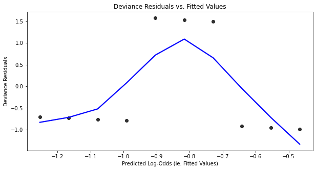
In general, we say that the more this fitted lowess curve in the fitted values vs. deviance residuals plot resembles...
- a horizontal line,
- with a y-intercept of 0
...the more that the training dataset meets the linearity assumption of the logistic regression model.
For instance, in the plot above we can definitely see that this lowess curve does not meet these two conditions. Thus, this indicates that the linearity assumption for the corresponding logistic regression model is not met. Or in other words, there is not a linear relationship between $x$ and the log-odds that $y=1$ in this dataset.
Instagram Logistic Regression Linearity Assumption
On the other hand, let's check this linearity assumption for our full Instagram logistic regression model.
By creating our fitted values vs. deviance residuals plot for the full model below, we do see a lowess curve that is much closer to resembling a horizontal line with a y-intercept at 0. Thus, we can say that this linearity assumption is much closer to being met for this logistic regression model and that this dataset is much closer to having a linear relationship between the 6 explanatory variables all together and the log-odds of an account being real.
plt.figure(figsize=(10,10))
sns.regplot(log_mod_full.fittedvalues, log_mod_full.resid_dev,
            color="black",
            line_kws={"color":"b"}, lowess=True)

plt.title("Deviance Residuals vs. Fitted Values")
plt.xlabel("Predicted Log-Odds (ie. Fitted Values)")
plt.ylabel("Deviance Residuals")
plt.show()
Assessing the Predictive Power of Just the Logistic Regression Model
Logistic Regression by Itself is not a Classifier
Recall that our main research goal for our Instagram logistic regression model is to use it to classify whether an account is real (ie. y=1) or fake (ie. y=0). Unfortunately, our fitted logistic regression model does not actually predict these 0/1 values for us explicitly. Instead it just returns the predictive probability $\hat{p}$ that the given observation is real (ie. y=1).
$\hat{p}=\frac{1}{1+e^{-(\hat{\beta}_0+\hat{\beta}_1x_1+...+\hat{\beta}_px_p)}}$
Thus, in section 10 we'll discuss how we can build and evaluate the performance of an actual classifier that predicts 0/1 values. This classifier takes an extra step after we get calculate a predictive probability $\hat{p}$ with a logistic regression model.
However, even before introducing this additional classification step to our logistic regression model, we can first evaluate how well the logistic regression model predicts a given dataset (training, test, new, etc) by itself.
Why not use R^2?
In a linear regression model we used the $R^2=1=\frac{SSE}{SST}$ metric to do this. However, also in line with our discussions in 5.2, calculating SSE (the sum square of the residuals) does not make as much a sense when our "residual" $y_i-\hat{p}_i$ is one that compares a 0/1 value to a probability.
Pseudo R^2
Instead we can use what we call the pseudo R^2 value. There are actually many pseudo R^2 value formulations that exist in the literature. One of the formulations that most directly references the objective function that we are actually trying maximize when fitting a logistic regression model is the McFadden Pseudo R^2 value which is calculated as follows.
- $LLF_{full}$=optimal log-likelihood function value of the model that you are evaluating
- $LLF_{null}$=optimal log-likelihood function value of the model that only has an intercept (ie. the null model
Extracting the Pseudo R^2
You can calculate the McFadden Pseudo R^2 for the training dataset that was used to fit the logistic regression model using the .prsquared attribute.
log_mod_full.prsquared0.819789878245675
Or you can look it up in the .summary() output table for the logistic regression model (under 'Pseudo R-squ') as well.
log_mod_full.summary()| Dep. Variable: | y | No. Observations: | 84 |
|---|---|---|---|
| Model: | Logit | Df Residuals: | 77 |
| Method: | MLE | Df Model: | 6 |
| Date: | Fri, 28 Jul 2023 | Pseudo R-squ.: | 0.8198 |
| Time: | 19:14:32 | Log-Likelihood: | -10.385 |
| converged: | False | LL-Null: | -57.628 |
| Covariance Type: | nonrobust | LLR p-value: | 3.538e-18 |
| coef | std err | z | P>|z| | [0.025 | 0.975] | |
|---|---|---|---|---|---|---|
| Intercept | -37.4658 | 4.38e+04 | -0.001 | 0.999 | -8.58e+04 | 8.57e+04 |
| has_a_profile_pic[T.yes] | 30.7281 | 4.38e+04 | 0.001 | 0.999 | -8.57e+04 | 8.58e+04 |
| number_of_words_in_name | 2.5983 | 1.203 | 2.161 | 0.031 | 0.241 | 4.955 |
| num_characters_in_bio | 0.0874 | 0.053 | 1.646 | 0.100 | -0.017 | 0.192 |
| number_of_posts | -0.0060 | 0.014 | -0.426 | 0.670 | -0.033 | 0.021 |
| number_of_followers | 0.0252 | 0.009 | 2.779 | 0.005 | 0.007 | 0.043 |
| number_of_follows | -0.0046 | 0.002 | -2.142 | 0.032 | -0.009 | -0.000 |
Possibly complete quasi-separation: A fraction 0.44 of observations can be
perfectly predicted. This might indicate that there is complete
quasi-separation. In this case some parameters will not be identified.
Interpreting the Pseudo R^2
Let's consider what might be better vs. worse values for $R^2_{MC}=1-\frac{LLF_{full}}{LLF_{null}}$
The higher the $R^2_{MC}$, the better the model fits the data.
Let's explore why this is.
Ideal Scenario for $LLF_{full}$
$LLF_{full}$, for instance, in our Instagram example, is going to the be highest possible log-likelihood function value that we could achieve with our intercept and 6 slopes $\beta_0,...,\beta_7$.
To recap, it represents the log() of the the product of all the probabilities of our response variable values $y_1,...,y_n$ in our dataset given the model and the set of explanatory variable values $\mathbf{x}_1,...,\mathbf{x}_n$ in our dataset.
$LLF_{full}=\mathbf{log}\left[P(Y=y_1|\beta_0,...,\beta_7, \mathbf{x}_1)\cdot\ldots\cdot P(Y=y_n|\beta_0,...,\beta_7, \mathbf{x}_n)\right]$
The ideal scenario for our fitted model with respect to the training data is one in which EVERY individual probability $P(Y=y_i|\beta_0,...,\beta_7, \mathbf{x}_i)=1$.
This would lead to the following equations outcomes.
$LF_{full}=\left[P(Y=y_1|\beta_0,...,\beta_7, \mathbf{x}_1)\cdot\ldots\cdot P(Y=y_n|\beta_0,...,\beta_7, \mathbf{x}_n)\right]=1$
$LLF_{full}=\mathbf{log}\left[P(Y=y_1|\beta_0,...,\beta_7, \mathbf{x}_1)\cdot\ldots\cdot P(Y=y_n|\beta_0,...,\beta_7, \mathbf{x}_n)\right]=0$
And thus the ideal $LLF_{full}=0$.
Better Values for $LLF_{full}$
However, most likely at least one individual probability $P(Y=y_i|\beta_0,...,\beta_7, \mathbf{x}_i)<1$.
This would lead to the following inequality outcomes.
$LF_{full}=\left[P(Y=y_1|\beta_0,...,\beta_7, \mathbf{x}_1)\cdot\ldots\cdot P(Y=y_n|\beta_0,...,\beta_7, \mathbf{x}_n)\right]<1$
$LLF_{full}=\mathbf{log}\left[P(Y=y_1|\beta_0,...,\beta_7, \mathbf{x}_1)\cdot\ldots\cdot P(Y=y_n|\beta_0,...,\beta_7, \mathbf{x}_n)\right]<0$
And thus realistically $LLF_{full}<0$.
Thus, $LLF_{full}$ will never be positive, but the closer this value is to 0, the better the fit for the training dataset.
Better Interpretation
For interpretation purposes, you can use the McFadden Pseudo-R^2 to standardize this $LLF_{full}$ by dividing by the the best log likelihood value $LLF_{null}$ you would get with the model that has just the intercept.
$R^2_{MC}=1-\frac{LLF_{full}}{LLF_{null}}$
Ideally, our logistic regression model that we're considering (ie. the "full model") should bring a lot of improvement to the objective function than what just the intercept model brought. Or in other words, the magnitude of $LLF_{full}$ should be a lot smaller than $LLF_{null}$. If this is the case, then $R^2_{MC}$ will become larger and approach 1.
However, given that we divided $LLF_{full}$ by $LLF_{null}$, it might be tempting to say that $R^2_{MC}$ is a relative metric. But unfortunately it is not! This means that you can not meaningfully compare the $R^2_{MC}$ of a model fit to one dataset to the $R^2_{MC}$ of a model fit to another dataset.
However, this metric is often used to compare the fit of multiple models for the same dataset.
Using the Pseudo R^2
For instance, the pseudo R^2=0.8198 for our full Instagram logistic regression model. Let's compare what happens to our pseudo R^2 when we (one at a time) take away each of our explanatory variables.
test_mod = smf.logit(formula='y~number_of_words_in_name+num_characters_in_bio+number_of_posts+number_of_followers+number_of_follows', data=df_train).fit(disp=False)
print('Removing has_a_profile_pic:',test_mod.prsquared)

test_mod = smf.logit(formula='y~has_a_profile_pic+num_characters_in_bio+number_of_posts+number_of_followers+number_of_follows', data=df_train).fit(disp=False)
print('Removing number_of_words_in_name:',test_mod.prsquared)

test_mod = smf.logit(formula='y~has_a_profile_pic+number_of_words_in_name+number_of_posts+number_of_followers+number_of_follows', data=df_train).fit(disp=False)
print('Removing num_characters_in_bio:',test_mod.prsquared)

test_mod = smf.logit(formula='y~has_a_profile_pic+number_of_words_in_name+num_characters_in_bio+number_of_followers+number_of_follows', data=df_train).fit(disp=False)
print('Removing number_of_posts:',test_mod.prsquared)

test_mod = smf.logit(formula='y~has_a_profile_pic+number_of_words_in_name+num_characters_in_bio+number_of_posts+number_of_follows', data=df_train).fit(disp=False)
print('Removing number_of_followers:',test_mod.prsquared)

test_mod = smf.logit(formula='y~has_a_profile_pic+number_of_words_in_name+num_characters_in_bio+number_of_posts+number_of_followers', data=df_train).fit(disp=False)
print('Removing number_of_follows:',test_mod.prsquared)
Removing has_a_profile_pic: 0.7230933052236868
Removing number_of_words_in_name: 0.7593630467603463
Removing num_characters_in_bio: 0.7723898648269075
Removing number_of_posts: 0.8185143541316554
Removing number_of_followers: 0.6395439976151506
Removing number_of_follows: 0.7342802891167286
Just like in a linear regression with R^2, if we remove an explanatory variable from the model, then our pseudo R^2 won't get any better (ie. higher).
But what we can see is that by removing number_of_posts variable, the pseudo R^2=0.8185 is only decreased by a small amount. Therefore, if our goal was to achieve a high fit of the training data, but we needed to remove at least one variable, we might consider removing number_of_posts as it only decreases the fit by a small amount.
Assessing the Predictive Power of the Logistic Regression Model used as a Classifier
As we'll discuss in section 10, by applying an extra step to our logistic regression predictive probability $\hat{p}_i$ for a given set of explanatory variable value inputs $\mathbf{x}_i$, we can actually classify this input as either a y=1 or y=0.
There's actually infinitely many classifiers that you could create from just a single logistic regression model. Therefore in section 10 we'll discuss more about how you can evaluate two distinct things.
- A specific classifier that a given logistic regression model has created.
- How well the logistic regression model will perform for all classifiers that could be created with it.
Trusting your Model Predictions
To recap from 7.4. we also discussed how in order to trust our model predictions, we should be careful not to extrapolate.
df_train[num_cols].describe().loc[['min','max']]| number_of_words_in_name | num_characters_in_bio | number_of_posts | number_of_followers | number_of_follows | |
|---|---|---|---|---|---|
| min | 0.0 | 0.0 | 0.0 | 0.0 | 1.0 |
| max | 5.0 | 138.0 | 590.0 | 1572.0 | 4239.0 |
When writing about and/or presenting a model that you plan to promote and use for it's predictive power, you should be upfront about the types of observations that you do not trust your model to perform well for.
For instance, we should be upfront with our readers that they should not try to predict accounts whose values fall outside of the explanatory variable ranges shown above.
For instance, we should NOT be using this model to predict whether or not Taylor Swift's Instagram account is real, her having 269 million followers (as of 7/24/2023).
Trusting your Model Slope Interpretations
Watch out for multicollinearity!
Finally, like with a linear regression model, in order to trust the interpretations of our logistic regression slopes, ideally our explanatory variables should not exhibit multicollinearity.
Similar to a linear regression model, having collinear explanatory variables in a logistic regression model can lead to biased slope interpretations.
In addition, collinear explanatory variables increase the chance that the model has been overfit to the training dataset. Given that our goal is to use our logistic regression model to predict whether an Instagram account is real or fake for new datasets, not overfitting is extremely important to us.
Fortunately, we saw in 2.2.3 no strong multicollinearity.
sns.pairplot(df_train[num_cols])
plt.show()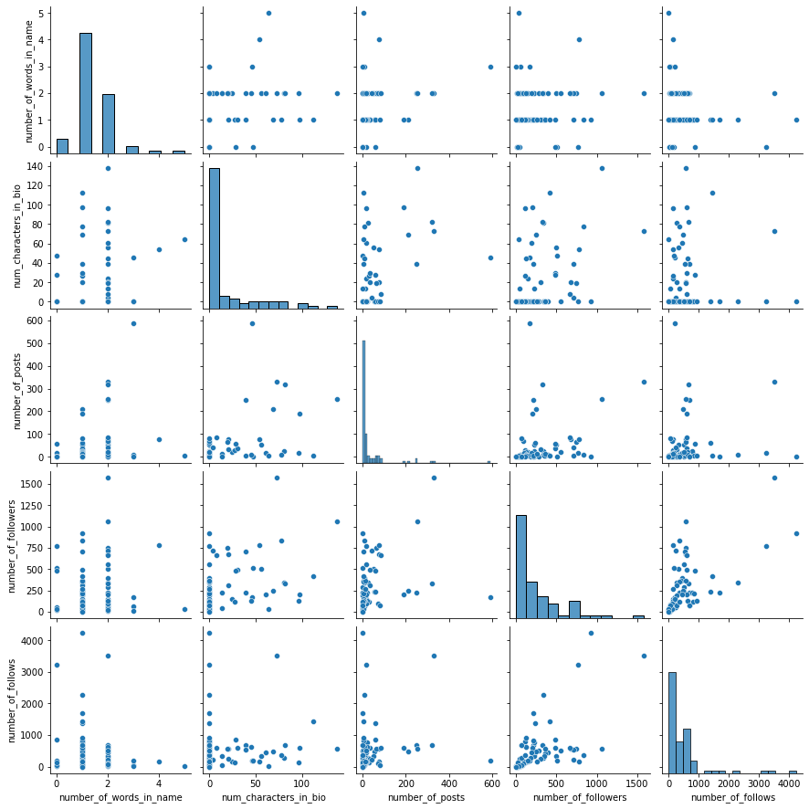
df_train[num_cols].corr()| number_of_words_in_name | num_characters_in_bio | number_of_posts | number_of_followers | number_of_follows | |
|---|---|---|---|---|---|
| number_of_words_in_name | 1.000000 | 0.310991 | 0.293882 | 0.126224 | -0.135021 |
| num_characters_in_bio | 0.310991 | 1.000000 | 0.500278 | 0.453310 | 0.119022 |
| number_of_posts | 0.293882 | 0.500278 | 1.000000 | 0.352771 | 0.179189 |
| number_of_followers | 0.126224 | 0.453310 | 0.352771 | 1.000000 | 0.619916 |
| number_of_follows | -0.135021 | 0.119022 | 0.179189 | 0.619916 | 1.000000 |
Watch out when interpreting slope magnitude!
Also, just like in a linear regression model you want to be careful about how/when you interpret the magnitude of a slope in a logistic regression model.
$
\hat{p} = \frac{1}{1 + \exp\left(-\begin{aligned}
&-37.47 \
&+ 30.73(,\text{has a profile pic}[T.yes]) \
&+ 2.60(,\text{number of words in name}) \
&+ 0.087(,\text{num characters in bio}) \
&- 0.0060(,\text{number of posts}) \
&+ 0.025(,\text{number of followers}) \
&- 0.0046(,\text{number of follows})
\end{aligned}\right)}
$
Take a look at our full logistic regression model above. We can see that the absolute value of the number_of_words_in_name slope (2.60) is much larger than the absolute value of the number_of_posts slope (-0.006). Does this mean that the number of words in an account name is more important when it comes to predicting whether or not an account is fake than the number of posts the account has made?
Not necessarily! Notice how the number_of_posts variable values tend to be a lot larger than the number_of_words_in_name variable values. As such, an increase of 1 post an account makes is not a large difference, when compared to an increase of 1 word in the account name.
As such, if these two variables had the same slope this would imply that that number_of_posts had a GREAT impact on the likelihood of the account being real, because such a comparatively small increase in the number of posts would dramatically increase the odds.
Thus, when the scales of the explanatory variables are not roughly all the same, you cannot interpret the magnitude of the slope as the importance of the variable when it comes to predicting the response variable.
On the other hand, if you scale your explanatory variables first to all have the same mean and standard deviation, then you can make this interpretation (provided that you're watching out for other slope interpretation issues like multicollinearity).
df_train[['number_of_words_in_name', 'number_of_posts']].describe().loc[['mean','std']]| number_of_words_in_name | number_of_posts | |
|---|---|---|
| mean | 1.369048 | 39.142857 |
| std | 0.818164 | 91.375716 |