Regularization Techniques
Similar to the backwards elimination algorithm and the forward selection algorithm, regularization techniques are another way to go about determining which explanatory variables may lead to overfitting and/or don't bring enough "predictive power" to the model, and should therefore be left out.
Introducing a Penalty Term into a Linear Regression
Similarity to Adjusted R^2 Metric
Similar to the adjusted R^2 metric, which we tried to maximize in our backwards elimination algorithm and the forward selection algorithm, these regularization techniques also introduce a type of penalty term that penalizes models that have too many explanatory variables that don't bring enough predictive power to the model.
In our adjusted R^2 equation, the penalty term was $(\frac{n-1}{n-p-1})$
$$Adjusted \ R^2=1-(\frac{SSE}{SST})\cdot(\frac{n-1}{n-p-1})$$
Adding More Slopes
Similarly, by increasing the number of slopes $p$, the adjusted R^2 will be encouraged to decrease. However, if we were to add a slope and the resulting decrease in the new model's error (SSE) were to be "large enough", then the adjusted R^2 would actually increase overall, and thus:
- this resulting model would be deemed "more parsimonious",
- this new slope would be considered bringing enough "predictive power" to the model, and
- this new slope would not be considered overfitting.
However, unfortunately, the quest of trying to find the linear regression model with the highest adjusted R^2 in the backwards elimination algorithm and the forward selection algorithms involved having to fit multiple models, each time checking the adjusted R^2 of the test models to see if the adjusted R^2 value got any better.
Objective Function
Modifying the Objective Function with a Penalty Term
So, rather than having to fit multiple basic linear regression models (and thus having to optimize multiple basic linear regression objective functions in search of the model that gives you the highest adjusted R^2), wouldn't it be great if we could just incorporate a penalty term directly into linear regression objective function?
This is the idea behind how a regularized linear regression model works. In a regularized linear regression model, we take the objective function from our basic (ie. nonregularized) linear regression model and add a type of penalty term.
Goal of the Penalty Term
So what specifically should we set this penalty term to be? Remember, the overall goal of our feature selection techniques is to determine which explanatory variables may cause our model to overfit to the training dataset, and therefore to determine which explanatory should we leave out of the model.
Goal 1: Interpretation of what to leave out
Question: So using just our regularized linear regression optimization problem above, what kind of optimal slope results could we get back that signals to us that the corresponding explanatory variable (or indicator variable) should be left out of the model?
Answer: If a returned optimal slope value is set $\hat{\beta}^*_i=0$, this serves as pretty clear signal that the model thinks the corresponding explanatory variable (or indicator variable) $x_i$ should be left out!
Goal 2: Leave out variables that lead to overfitting
Questions: Now that we know how our fitted regularized linear regression model will indicate to us which variables should be left out, how should we set up this penalty term to encourage the model to only indicate leaving out the variables that lead to "too much" overfitting? Furthermore, how do we define "too much" overfitting?
Answers: In sections 8.2, 8.3, and 8.4 we'll talk about three of the most popular penalty term functions that are used that attempt to satisfy these two goals.
- 8.2. L1 Penalty Term (ie. LASSO Regression)
- 8.3. L2 Penalty Term (ie. Ridge Regression)
- 8.4 Combination of L1 and L2 Penalty Terms (ie. Elastic Net Regression)
LASSO Regression (ie. L1 Penalty Term)
In the regularized LASSO linear regression optimization problem shown below, the penalty term that is added is
We call this a L1 penalty term, because what we call the L1 norm of a given list (ie. vector) of values is the sum of the absolute values of the values in this list. (The LASSO stands for Least Absolute Shrinkage and Selection Operator).
Also in this penalty term, we introduce a parameter $\lambda\geq 0$ that we need to choose ahead of time. This $\lambda$ value can be anything you want as long as it is not negative.
The Ideal Scenario
To help us see why adding this penalty term would help to reduce overfitting, let's think about what the absolute best intercept and slope solutions to this optimization would be. We can see that the full objective function now is comprised of the sum of two terms.
- $SSE=\left[ \sum_{i=1}^n(y_i-(\hat{\beta}_0+\hat{\beta}_1x_{i,1}+...+\hat{\beta}_{50}x_{i,50}))^2 \right]$
- $\lambda\cdot\left[|\hat{\beta}_1|+|\hat{\beta}_2|+...+|\hat{\beta}_{50}|\right]$
The Penalty Term Balancing Act
However, note that this "ideal scenario" that we just described is unrealistic. It's unlikely that we'll be able to fit a model where ALL the slopes $\hat{\beta}_j=0$ AND there is absolutely NO model error (ie. $SSE=0$). In addition, what we actually see is that these terms end up competing with one another. That is, choosing intercepts and slopes that lead to a decrease of one term, often leads to an increase in the other term, and vice versa.
The Impact of $\lambda$
Now let's think about the impact that our preselected $\lambda$ parameter has on this balancing act.
If we were to set $\lambda$ to be as low as possible (=0), then we can see that this penalty term would actually have no impact at all on the linear regression intercepts and slopes that were chosen. With $\lambda=0$, then we can see that our objective function actually just becomes the same as our nonregularized linear regression objective function. Thus in this case, we are fitting just a basic linear regression model. The slopes values face no penalty for being as large as they need to be in order to minimize the SSE.
Which slope magnitudes get to stay large?
But does this mean that all of the $|\hat{\beta}_j|$ terms need to decrease equally? Or is it possible that the optimization problem will cleverly keep some slopes high that correspond to the variables that contribute the most predictive power to the model thereby leading to much larger reductions to the SSE? And could it also keep other slopes low that correspond to the variables that do not contribute a lot independently to the predictive power of the model (or in other words, may be causing the model to overfit)? Luckily, in practice we see that the answer to these questions is yes!
Thus the resulting optimal slopes that are set low, are the ones that bring the least predictive power to the model and thus are the most likely variable to overfit the model.
Clearer Slope Interpretation with LASSO Regression
So what we learned is that the less predictive power that a given variable independently brings to a regression model, the more likely it's corresponding slope is going to be set low. But then we might ask: how do we know if a resulting slope value is low enough to warrant leaving it out of the model because it does not bring enough predictive power to the model?
One of the benefits of using the L1 penalty term in regression regularization (as opposed to the other two penalty terms that we'll discuss in 8.3 and 8.4) is how the absolute value function interacts with our Calculus techniques that are used to solve for these optimal intercept and slope solutions. In general, if a slope is encouraged by the optimization problem to be comparatively small, then the optimal solution values for these small slopes can actually force these small slope values to be set exactly equal to 0.
These small slope values being set exactly equal to 0, gets rid of a lot of the interpretation ambiguity. If a slope is set to be 0, then the LASSO regression model is suggesting that this slope's corresponding variable can be left out of the model because it is not bringing enough predictive power to the model, based on the $\lambda$ value that you chose.
Nonregularized Linear Regression for Predicting Tumor Size - for Comparison
Before we fit a LASSO linear regression model with our scaled training features matrix and target array, let's also fit a basic nonregularized linear regression model for comparison purposes. To do so, let's use the LinearRegression() that we used in Data Science Discovery.
Recall that we first instantiate an object with this LinearRegression() function. And then we use the .fit() function with our features matrix ($X_{train}$) and target array ($y_{train}$) to actually fit the model.
from sklearn.linear_model import LinearRegression

lin_reg_mod = LinearRegression()
lin_reg_mod.fit(X_train, y_train)LinearRegression()In a Jupyter environment, please rerun this cell to show the HTML representation or trust the notebook.
On GitHub, the HTML representation is unable to render, please try loading this page with nbviewer.org.
LinearRegression()
And let's display the slopes for this fitted linear regression model below by using the .coef_ attribute. Because we scaled our gene explanatory variables, we are technically able to interpret the corresponding slope magnitudes as an indication of how important that particular corresponding variable is when it comes to predicting the tumor size in this particular model, in the context of the other existing variables in the model.
df_slopes = pd.DataFrame(lin_reg_mod.coef_.T, columns = ['lin_reg_mod'], index=X_train.columns)
df_slopes.sort_values(by=['lin_reg_mod'])| lin_reg_mod | |
|---|---|
| X1595 | -23.334004 |
| X980 | -10.996647 |
| X1169 | -10.944499 |
| X1470 | -10.656927 |
| X1193 | -6.094789 |
| X1141 | -5.867328 |
| X1563 | -4.857389 |
| X1203 | -4.274063 |
| X1023 | -3.991874 |
| X1506 | -3.580033 |
| X986 | -3.413999 |
| X1264 | -3.258595 |
| X1514 | -2.879311 |
| X1416 | -1.948134 |
| X1656 | -1.881983 |
| X1637 | -1.837732 |
| X1219 | -1.244601 |
| X1657 | -1.060942 |
| X1417 | -0.923660 |
| X1103 | -0.739345 |
| X1418 | -0.726373 |
| X1529 | -0.556923 |
| X1136 | -0.547525 |
| X1232 | -0.493502 |
| X1092 | -0.408996 |
| X1109 | 0.121617 |
| X1553 | 0.126864 |
| X1124 | 0.488547 |
| X1144 | 0.657140 |
| X1444 | 0.971105 |
| X1179 | 1.212503 |
| X1597 | 1.487872 |
| X1683 | 1.749397 |
| X1206 | 1.790304 |
| X1064 | 2.006906 |
| X159 | 2.093903 |
| X1609 | 2.157559 |
| X1351 | 2.802728 |
| X1028 | 3.797146 |
| X1362 | 3.868178 |
| X1208 | 4.107494 |
| X1292 | 4.623105 |
| X1272 | 6.584962 |
| X1574 | 7.214710 |
| X1173 | 7.801992 |
| X1297 | 8.719397 |
| X960 | 9.995326 |
| X1329 | 11.802248 |
| X1430 | 12.056850 |
| X1616 | 13.586829 |
Issue #1: Biased Slopes due to Multicollinearity
However, remember that our features matrix showed many pairs of variables that were collinear. Thus, it is possible that our slope interpretations could still be biased due to this multicollinearity.
Issue #2: Could we be Overfitting?
Remember that one of our other goals is to use our predictive model to attain good predictions for new datasets. Let's assess the test dataset $R^2$ of this linear regression model before moving on to our LASSO linear regression model.
We can use the .score() function along with our test features matrix $X_{test}$ and target array $y_{test}$ to calculate this test R^2 of the model.
lin_reg_mod.score(X_test, y_test)-0.3071595344334954
Negative R^2?
Interestingly enough we got a $R^2$ value that may not be what we were expecting. The R^2 of the test dataset is negative for this model! If the R^2 value was between 0 and 1, this value would represent the percent of tumor size variability that is explained by the model.
However, when the R^2 value is negative, one downside is that we lose the interpretability. Another huge downside, is that this implies that this model is a not a good fit for the test dataset. In general, the lower the R^2 value, the worse the fit.
LASSO Linear Regression for Predicting Tumor Size
Now, let's actually apply our LASSO Linear regression model to this dataset.
Recall that our LASSO linear regression objective function required for us to preselect a value for $\lambda$. Let's try out a couple different values for $\lambda\in [0.025, 0.05, 0.1, 0.5]$ and see how this impacts our results and research goals.
We can use the Lasso() function to fit a linear LASSO regression model. This Lasso() function operates in a similar way to the LinearRegression() function. First, we create a Lasso() object with specified parameters. Then we take this object and .fit() it with the features matrix and the target array.
- The alpha parameter represents the $\lambda$ parameter.
- The algorithm that is used to attempt to find the optimal intercept and slopes to this LASSO regression objective function may not always arrive at an optimal solution in a fixed number of steps. Therefore, in the interest of time, we can set the max_iter parameter to be the maximum number of iterations that this algorithm should take before just stopping early and returning the best solution that it currently has.
Fitting Four LASSO Models
Model 1: $\lambda=0.025$
from sklearn.linear_model import Lasso
lasso_mod_025 = Lasso(alpha=0.025, max_iter=1000)
lasso_mod_025.fit(X_train, y_train)Lasso(alpha=0.025)In a Jupyter environment, please rerun this cell to show the HTML representation or trust the notebook.
On GitHub, the HTML representation is unable to render, please try loading this page with nbviewer.org.
Lasso(alpha=0.025)
Model 2: $\lambda=.05$
lasso_mod_05 = Lasso(alpha=.05, max_iter=1000)
lasso_mod_05.fit(X_train, y_train)Lasso(alpha=0.05)In a Jupyter environment, please rerun this cell to show the HTML representation or trust the notebook.
On GitHub, the HTML representation is unable to render, please try loading this page with nbviewer.org.
Lasso(alpha=0.05)
Model 3: $\lambda=.1$
lasso_mod_1 = Lasso(alpha=.1, max_iter=1000)
lasso_mod_1.fit(X_train, y_train)Lasso(alpha=0.1)In a Jupyter environment, please rerun this cell to show the HTML representation or trust the notebook.
On GitHub, the HTML representation is unable to render, please try loading this page with nbviewer.org.
Lasso(alpha=0.1)
Model 4: $\lambda=.5$
lasso_mod_5 = Lasso(alpha=.5, max_iter=1000)
lasso_mod_5.fit(X_train, y_train)Lasso(alpha=0.5)In a Jupyter environment, please rerun this cell to show the HTML representation or trust the notebook.
On GitHub, the HTML representation is unable to render, please try loading this page with nbviewer.org.
Lasso(alpha=0.5)
Inspecting the Slopes
Next, let's inspect and compare the slopes of the models that we've created so far. We can similarly using the .coef attribute to extract each of our 4 model slopes.
By comparing the slopes of the four LASSO linear regression models, we can see what we would expect. As we increase $\lambda$, the number of non-zero slopes decreased. In fact, when $\lambda=0.5$, there were only seven genes with non-zero slopes. This result may suggest that these genes are the most important when it comes to predicting breast tumor size.
df_slopes = pd.DataFrame({'lin_reg_mod': lin_reg_mod.coef_.T,
                         'lasso_mod_025': lasso_mod_025.coef_.T,
                         'lasso_mod_05': lasso_mod_05.coef_.T,
                         'lasso_mod_1': lasso_mod_1.coef_.T,
                         'lasso_mod_5': lasso_mod_5.coef_.T}, index=X_train.columns)
df_slopes| lin_reg_mod | lasso_mod_025 | lasso_mod_05 | lasso_mod_1 | lasso_mod_5 | |
|---|---|---|---|---|---|
| X159 | 2.093903 | 1.452509 | 1.098574 | 0.593176 | 0.000000 |
| X960 | 9.995326 | 8.302795 | 6.596317 | 4.266726 | 0.000000 |
| X980 | -10.996647 | -7.199944 | -4.237265 | -0.704563 | -0.000000 |
| X986 | -3.413999 | -2.592459 | -1.775948 | -0.000000 | -0.000000 |
| X1023 | -3.991874 | -3.340229 | -2.766260 | -2.092078 | -0.147790 |
| X1028 | 3.797146 | 3.196267 | 2.871440 | 2.605532 | 1.912208 |
| X1064 | 2.006906 | 2.341590 | 2.206635 | 1.691021 | 0.000000 |
| X1092 | -0.408996 | -0.338999 | -0.259970 | -0.234224 | 0.000000 |
| X1103 | -0.739345 | -0.000000 | -0.000000 | 0.000000 | -0.000000 |
| X1109 | 0.121617 | -0.789248 | -2.023169 | -2.986337 | -0.000000 |
| X1124 | 0.488547 | 0.000000 | -0.000000 | -0.000000 | 0.000000 |
| X1136 | -0.547525 | -0.206065 | -0.000000 | -0.000000 | -0.673779 |
| X1141 | -5.867328 | -5.052785 | -4.416822 | -2.981458 | -0.481311 |
| X1144 | 0.657140 | 0.126505 | 0.000000 | -0.000000 | 0.000000 |
| X1169 | -10.944499 | -5.637134 | -3.492767 | -0.986729 | -0.000000 |
| X1173 | 7.801992 | 5.701120 | 3.886316 | 1.669699 | -0.000000 |
| X1179 | 1.212503 | 0.711820 | 0.473037 | 0.412424 | -0.000000 |
| X1193 | -6.094789 | -4.625321 | -2.528730 | -0.000000 | -0.000000 |
| X1203 | -4.274063 | -1.917869 | -0.418720 | -0.000000 | -0.000000 |
| X1206 | 1.790304 | 1.148111 | 0.786031 | 0.216690 | 0.000000 |
| X1208 | 4.107494 | 3.441126 | 2.072339 | 0.342848 | 0.000000 |
| X1219 | -1.244601 | -0.852432 | -0.968064 | -0.850370 | -0.000000 |
| X1232 | -0.493502 | -0.000000 | -0.000000 | -0.000000 | 0.000000 |
| X1264 | -3.258595 | -2.175231 | -1.305576 | -0.045646 | -0.000000 |
| X1272 | 6.584962 | 2.679780 | 0.528721 | 0.000000 | -0.000000 |
| X1292 | 4.623105 | 0.675658 | 0.000000 | -0.000000 | -0.000000 |
| X1297 | 8.719397 | 1.117108 | 0.000000 | 0.000000 | -0.000000 |
| X1329 | 11.802248 | 8.539188 | 5.536811 | 0.918378 | -0.000000 |
| X1351 | 2.802728 | 1.551829 | 0.466324 | -0.000000 | -0.009818 |
| X1362 | 3.868178 | 2.878842 | 2.239372 | 0.875101 | -0.000000 |
| X1416 | -1.948134 | -1.688431 | -1.259215 | -0.933760 | -0.284509 |
| X1417 | -0.923660 | -0.825183 | -0.432391 | -0.479412 | -0.000000 |
| X1418 | -0.726373 | -0.371522 | -0.000000 | -0.000000 | -0.000000 |
| X1430 | 12.056850 | 9.071478 | 7.372312 | 5.274174 | 0.000000 |
| X1444 | 0.971105 | 0.894966 | 0.609778 | 0.000000 | 0.000000 |
| X1470 | -10.656927 | -7.210662 | -5.213523 | -2.155941 | -0.000000 |
| X1506 | -3.580033 | -1.160591 | -0.255748 | -0.000000 | -0.000000 |
| X1514 | -2.879311 | -2.347902 | -2.106235 | -2.149132 | -0.730586 |
| X1529 | -0.556923 | -0.321777 | -0.328990 | -0.380970 | -0.000000 |
| X1553 | 0.126864 | -0.000000 | -0.000000 | -0.000000 | 0.000000 |
| X1563 | -4.857389 | -3.100188 | -2.107724 | -1.007217 | -0.000000 |
| X1574 | 7.214710 | 0.000000 | -0.000000 | -0.000000 | 0.000000 |
| X1595 | -23.334004 | -1.343896 | -1.080912 | -0.000000 | 0.000000 |
| X1597 | 1.487872 | 0.420259 | -0.000000 | -0.126035 | -0.000000 |
| X1609 | 2.157559 | 1.912054 | 1.368465 | 0.826883 | 0.000000 |
| X1616 | 13.586829 | -0.000000 | -0.000000 | -0.571179 | -0.000000 |
| X1637 | -1.837732 | -0.810217 | -0.103097 | -0.000000 | -0.000000 |
| X1656 | -1.881983 | -1.962349 | -1.742366 | -1.070309 | -0.000000 |
| X1657 | -1.060942 | -0.122512 | -0.000000 | -0.000000 | -0.000000 |
| X1683 | 1.749397 | 1.144410 | 0.469739 | 0.000000 | -0.000000 |
Which model is best?
But could it be possible that some of these LASSO models have left out too many explanatory variables and thus may be underfitting?
Given that one of our goals is to build a model that will yield good predictions for new breast tumors, let's inspect the test dataset R^2 of each of these 4 LASSO models.
Nonregularized Linear Regression Model: Test Dataset R^2
lin_reg_mod.score(X_test, y_test)-0.3071595344334954
LASSO Model 1: $\lambda=0.025$ Test Dataset R^2
lasso_mod_025.score(X_test, y_test)0.1539346136658848
LASSO Model 2: $\lambda=0.05$ Test Dataset R^2
lasso_mod_05.score(X_test, y_test)0.2786886369663709
LASSO Model 3: $\lambda=0.1$ Test Dataset R^2
lasso_mod_1.score(X_test, y_test)0.2490838650434536
LASSO Model 4: $\lambda=0.5$ Test Dataset R^2
lasso_mod_5.score(X_test, y_test)0.1445914387347873
We can see that the linear regression model that achieves the best test dataset R^2=0.279 is the LASSO model that used $\lambda=0.05$. Ideally, a more complete analysis would try out many other values of $\lambda$ to see if we can find a test dataset R^2 that was even higher.
Can we trust the non-zero slope interpretations in our chosen LASSO model?
Ideally, we'd be able to trust our interpretations of our non-zero slopes in this resulting LASSO model that we chose as well. Recall that many of our 50 gene explanatory variables in the nonregularized linear regression model were collinear with each other, which should make us more skeptical about how we interpret the resulting slopes.
If we were to remove the explanatory variables that had zero slopes in our chosen LASSO model, would the remaining explanatory variables still be collinear?
Below is a list of the 37 gene names that had non-zero slopes in our best LASSO model.
nonzero_slope_genes = df_slopes[np.abs(df_slopes['lasso_mod_05'])>0.00001].index
nonzero_slope_genes
Index(['X159', 'X960', 'X980', 'X986', 'X1023', 'X1028', 'X1064', 'X1092',
'X1109', 'X1141', 'X1169', 'X1173', 'X1179', 'X1193', 'X1203', 'X1206',
'X1208', 'X1219', 'X1264', 'X1272', 'X1329', 'X1351', 'X1362', 'X1416',
'X1417', 'X1430', 'X1444', 'X1470', 'X1506', 'X1514', 'X1529', 'X1563',
'X1595', 'X1609', 'X1637', 'X1656', 'X1683'],
dtype='object')
And below is the correlation matrix of each of these 37 remaining genes.
X_train_remaining = X_train[nonzero_slope_genes]
X_train_remaining.corr()| X159 | X960 | X980 | X986 | X1023 | X1028 | X1064 | X1092 | X1109 | X1141 | ... | X1470 | X1506 | X1514 | X1529 | X1563 | X1595 | X1609 | X1637 | X1656 | X1683 | |
|---|---|---|---|---|---|---|---|---|---|---|---|---|---|---|---|---|---|---|---|---|---|
| X159 | 1.000000 | 0.060265 | -0.065454 | 0.022752 | 0.002266 | -0.226498 | -0.035437 | -0.160238 | -0.110140 | 0.011729 | ... | 0.043124 | -0.031407 | -0.086193 | 0.262708 | 0.146743 | -0.010273 | -0.141372 | -0.072578 | 0.134411 | -0.151282 |
| X960 | 0.060265 | 1.000000 | -0.916792 | 0.919474 | 0.864897 | -0.656544 | 0.934777 | -0.444383 | -0.882282 | 0.871462 | ... | 0.927974 | -0.927604 | -0.820769 | 0.807609 | 0.888604 | -0.851930 | -0.841161 | -0.825226 | 0.793374 | -0.838848 |
| X980 | -0.065454 | -0.916792 | 1.000000 | -0.863944 | -0.775288 | 0.762141 | -0.913493 | 0.513205 | 0.948234 | -0.864145 | ... | -0.941770 | 0.977642 | 0.820674 | -0.866144 | -0.883796 | 0.874294 | 0.873856 | 0.895619 | -0.860707 | 0.893986 |
| X986 | 0.022752 | 0.919474 | -0.863944 | 1.000000 | 0.810531 | -0.650212 | 0.909173 | -0.449640 | -0.805998 | 0.829365 | ... | 0.906335 | -0.886268 | -0.755153 | 0.736371 | 0.855282 | -0.826968 | -0.794439 | -0.786007 | 0.716178 | -0.804646 |
| X1023 | 0.002266 | 0.864897 | -0.775288 | 0.810531 | 1.000000 | -0.618030 | 0.789146 | -0.379213 | -0.712516 | 0.756040 | ... | 0.785812 | -0.788302 | -0.685370 | 0.682320 | 0.762159 | -0.787609 | -0.708756 | -0.682828 | 0.638509 | -0.662923 |
| X1028 | -0.226498 | -0.656544 | 0.762141 | -0.650212 | -0.618030 | 1.000000 | -0.645414 | 0.484050 | 0.722887 | -0.651875 | ... | -0.707760 | 0.743441 | 0.683551 | -0.696159 | -0.706024 | 0.762429 | 0.725366 | 0.729037 | -0.659633 | 0.699566 |
| X1064 | -0.035437 | 0.934777 | -0.913493 | 0.909173 | 0.789146 | -0.645414 | 1.000000 | -0.485517 | -0.874262 | 0.861079 | ... | 0.926588 | -0.928034 | -0.837623 | 0.760780 | 0.860687 | -0.843057 | -0.823614 | -0.845297 | 0.776042 | -0.844329 |
| X1092 | -0.160238 | -0.444383 | 0.513205 | -0.449640 | -0.379213 | 0.484050 | -0.485517 | 1.000000 | 0.400143 | -0.469561 | ... | -0.455920 | 0.496425 | 0.470159 | -0.429428 | -0.516239 | 0.562968 | 0.522040 | 0.410890 | -0.441094 | 0.445237 |
| X1109 | -0.110140 | -0.882282 | 0.948234 | -0.805998 | -0.712516 | 0.722887 | -0.874262 | 0.400143 | 1.000000 | -0.812283 | ... | -0.900745 | 0.935573 | 0.798052 | -0.857029 | -0.822570 | 0.798974 | 0.822577 | 0.910524 | -0.848353 | 0.877479 |
| X1141 | 0.011729 | 0.871462 | -0.864145 | 0.829365 | 0.756040 | -0.651875 | 0.861079 | -0.469561 | -0.812283 | 1.000000 | ... | 0.868621 | -0.869839 | -0.736111 | 0.745264 | 0.843947 | -0.799305 | -0.782430 | -0.712398 | 0.799659 | -0.801396 |
| X1169 | -0.004202 | 0.925896 | -0.926571 | 0.864454 | 0.789092 | -0.699165 | 0.909802 | -0.447707 | -0.883932 | 0.924337 | ... | 0.923992 | -0.930818 | -0.786308 | 0.784502 | 0.867721 | -0.863700 | -0.846288 | -0.823758 | 0.820538 | -0.840337 |
| X1173 | 0.058787 | 0.903325 | -0.884817 | 0.870304 | 0.776981 | -0.693137 | 0.877916 | -0.554142 | -0.794434 | 0.909999 | ... | 0.880804 | -0.885603 | -0.791922 | 0.767329 | 0.863425 | -0.850215 | -0.833425 | -0.736912 | 0.749456 | -0.804784 |
| X1179 | 0.062648 | 0.737455 | -0.736313 | 0.654872 | 0.641327 | -0.605075 | 0.656605 | -0.343754 | -0.711082 | 0.775219 | ... | 0.737398 | -0.739159 | -0.511046 | 0.685649 | 0.740930 | -0.685372 | -0.635948 | -0.620235 | 0.763833 | -0.608884 |
| X1193 | 0.091274 | 0.933136 | -0.930017 | 0.873882 | 0.803894 | -0.673898 | 0.908863 | -0.465221 | -0.881124 | 0.893868 | ... | 0.907854 | -0.917627 | -0.771814 | 0.857625 | 0.887649 | -0.828686 | -0.830956 | -0.804668 | 0.809600 | -0.834385 |
| X1203 | 0.079657 | 0.916031 | -0.904998 | 0.899109 | 0.779479 | -0.687560 | 0.899677 | -0.485905 | -0.861692 | 0.861878 | ... | 0.938010 | -0.916234 | -0.724234 | 0.806315 | 0.910898 | -0.810954 | -0.803194 | -0.828396 | 0.828596 | -0.794665 |
| X1206 | 0.174463 | 0.760769 | -0.742724 | 0.796077 | 0.670605 | -0.639950 | 0.746090 | -0.500799 | -0.687160 | 0.741375 | ... | 0.771183 | -0.754391 | -0.642960 | 0.724521 | 0.802564 | -0.695499 | -0.656429 | -0.651239 | 0.666202 | -0.673853 |
| X1208 | 0.044885 | 0.908029 | -0.926673 | 0.884039 | 0.765225 | -0.671927 | 0.926455 | -0.450485 | -0.905937 | 0.877521 | ... | 0.930512 | -0.932100 | -0.767078 | 0.814237 | 0.879817 | -0.815426 | -0.795445 | -0.824524 | 0.834101 | -0.844577 |
| X1219 | 0.180275 | 0.769047 | -0.807458 | 0.769531 | 0.633759 | -0.633706 | 0.733670 | -0.411896 | -0.761748 | 0.752468 | ... | 0.851443 | -0.817103 | -0.559037 | 0.710085 | 0.830423 | -0.711176 | -0.705878 | -0.733160 | 0.800655 | -0.708285 |
| X1264 | -0.051055 | -0.781417 | 0.802760 | -0.782776 | -0.703112 | 0.658323 | -0.804180 | 0.397005 | 0.814639 | -0.648905 | ... | -0.757512 | 0.795819 | 0.771927 | -0.703418 | -0.681377 | 0.758941 | 0.786272 | 0.803112 | -0.603683 | 0.774020 |
| X1272 | -0.040265 | -0.911553 | 0.947765 | -0.873484 | -0.767387 | 0.751029 | -0.915850 | 0.494310 | 0.891946 | -0.866641 | ... | -0.937044 | 0.965954 | 0.849028 | -0.781977 | -0.865252 | 0.881443 | 0.847869 | 0.859305 | -0.817937 | 0.893305 |
| X1329 | 0.009951 | 0.929842 | -0.932724 | 0.886701 | 0.789396 | -0.695484 | 0.909363 | -0.441399 | -0.895399 | 0.940292 | ... | 0.954865 | -0.940787 | -0.778585 | 0.792883 | 0.904664 | -0.839982 | -0.830809 | -0.815080 | 0.867191 | -0.863806 |
| X1351 | 0.074195 | 0.811867 | -0.847300 | 0.750453 | 0.680455 | -0.660163 | 0.795969 | -0.450868 | -0.825490 | 0.831995 | ... | 0.843567 | -0.838437 | -0.692781 | 0.810342 | 0.861870 | -0.751341 | -0.743854 | -0.730542 | 0.850602 | -0.750289 |
| X1362 | 0.020027 | 0.918716 | -0.923671 | 0.875123 | 0.802120 | -0.676309 | 0.902487 | -0.419660 | -0.897589 | 0.869691 | ... | 0.923741 | -0.927871 | -0.724029 | 0.826481 | 0.887244 | -0.806308 | -0.808091 | -0.843427 | 0.835359 | -0.804713 |
| X1416 | 0.180052 | 0.383643 | -0.502941 | 0.356281 | 0.214178 | -0.423820 | 0.400211 | -0.473305 | -0.477921 | 0.480017 | ... | 0.436741 | -0.450760 | -0.351886 | 0.565908 | 0.502524 | -0.425664 | -0.416625 | -0.375468 | 0.593593 | -0.429165 |
| X1417 | -0.074155 | -0.891227 | 0.949137 | -0.835970 | -0.775966 | 0.776325 | -0.879697 | 0.439637 | 0.910556 | -0.832863 | ... | -0.897464 | 0.943863 | 0.839946 | -0.832228 | -0.830148 | 0.847958 | 0.872998 | 0.868016 | -0.804726 | 0.887542 |
| X1430 | -0.077804 | -0.891555 | 0.900095 | -0.830997 | -0.774981 | 0.675972 | -0.858329 | 0.479091 | 0.877924 | -0.803209 | ... | -0.826189 | 0.885129 | 0.839241 | -0.830799 | -0.788063 | 0.832096 | 0.837266 | 0.829237 | -0.717934 | 0.837409 |
| X1444 | -0.151062 | -0.822917 | 0.910982 | -0.774846 | -0.698487 | 0.763655 | -0.821939 | 0.516456 | 0.868480 | -0.774262 | ... | -0.848531 | 0.902977 | 0.790241 | -0.795023 | -0.779184 | 0.826656 | 0.814365 | 0.812694 | -0.760813 | 0.851153 |
| X1470 | 0.043124 | 0.927974 | -0.941770 | 0.906335 | 0.785812 | -0.707760 | 0.926588 | -0.455920 | -0.900745 | 0.868621 | ... | 1.000000 | -0.952881 | -0.771150 | 0.801664 | 0.923467 | -0.832105 | -0.836461 | -0.856976 | 0.863743 | -0.854665 |
| X1506 | -0.031407 | -0.927604 | 0.977642 | -0.886268 | -0.788302 | 0.743441 | -0.928034 | 0.496425 | 0.935573 | -0.869839 | ... | -0.952881 | 1.000000 | 0.828279 | -0.830340 | -0.892210 | 0.876923 | 0.846958 | 0.901064 | -0.843021 | 0.897225 |
| X1514 | -0.086193 | -0.820769 | 0.820674 | -0.755153 | -0.685370 | 0.683551 | -0.837623 | 0.470159 | 0.798052 | -0.736111 | ... | -0.771150 | 0.828279 | 1.000000 | -0.696167 | -0.724666 | 0.795717 | 0.783708 | 0.771904 | -0.647816 | 0.851241 |
| X1529 | 0.262708 | 0.807609 | -0.866144 | 0.736371 | 0.682320 | -0.696159 | 0.760780 | -0.429428 | -0.857029 | 0.745264 | ... | 0.801664 | -0.830340 | -0.696167 | 1.000000 | 0.808604 | -0.721919 | -0.781370 | -0.784322 | 0.794576 | -0.767723 |
| X1563 | 0.146743 | 0.888604 | -0.883796 | 0.855282 | 0.762159 | -0.706024 | 0.860687 | -0.516239 | -0.822570 | 0.843947 | ... | 0.923467 | -0.892210 | -0.724666 | 0.808604 | 1.000000 | -0.793890 | -0.774063 | -0.767569 | 0.851589 | -0.779229 |
| X1595 | -0.010273 | -0.851930 | 0.874294 | -0.826968 | -0.787609 | 0.762429 | -0.843057 | 0.562968 | 0.798974 | -0.799305 | ... | -0.832105 | 0.876923 | 0.795717 | -0.721919 | -0.793890 | 1.000000 | 0.829484 | 0.793389 | -0.702696 | 0.779285 |
| X1609 | -0.141372 | -0.841161 | 0.873856 | -0.794439 | -0.708756 | 0.725366 | -0.823614 | 0.522040 | 0.822577 | -0.782430 | ... | -0.836461 | 0.846958 | 0.783708 | -0.781370 | -0.774063 | 0.829484 | 1.000000 | 0.828017 | -0.722580 | 0.811844 |
| X1637 | -0.072578 | -0.825226 | 0.895619 | -0.786007 | -0.682828 | 0.729037 | -0.845297 | 0.410890 | 0.910524 | -0.712398 | ... | -0.856976 | 0.901064 | 0.771904 | -0.784322 | -0.767569 | 0.793389 | 0.828017 | 1.000000 | -0.739133 | 0.851905 |
| X1656 | 0.134411 | 0.793374 | -0.860707 | 0.716178 | 0.638509 | -0.659633 | 0.776042 | -0.441094 | -0.848353 | 0.799659 | ... | 0.863743 | -0.843021 | -0.647816 | 0.794576 | 0.851589 | -0.702696 | -0.722580 | -0.739133 | 1.000000 | -0.752078 |
| X1683 | -0.151282 | -0.838848 | 0.893986 | -0.804646 | -0.662923 | 0.699566 | -0.844329 | 0.445237 | 0.877479 | -0.801396 | ... | -0.854665 | 0.897225 | 0.851241 | -0.767723 | -0.779229 | 0.779285 | 0.811844 | 0.851905 | -0.752078 | 1.000000 |
37 rows × 37 columns
sns.heatmap(X_train_remaining.corr(),vmin=-1, vmax=1, cmap='RdBu')
plt.show()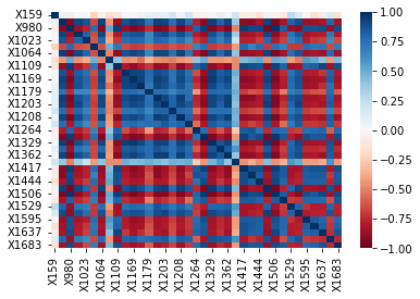
Unfortunately, there is still a high degree of multicollinearity in the remaining explanatory variables. Therefore, we should also be cautious when interpreting the slopes of our chosen LASSO model as well.
Ridge Regression (ie. L2 Penalty Term)
Similar to LASSO regression, we introduce a parameter $\lambda\geq 0$ that we must preselect.
The Ideal Scenario
Similar to the LASSO linear regression, the absolute best intercept and slope solutions to this optimization would be ones in which:
- $SSE=\left[ \sum_{i=1}^n(y_i-(\hat{\beta}_0+\hat{\beta}_1x_{i,1}+...+\hat{\beta}_{50}x_{i,50}))^2 \right]=0$
- $\lambda\cdot\left[|\hat{\beta}_1|+|\hat{\beta}_2|+...+|\hat{\beta}_{50}|\right]=0$
The Penalty Term Balancing Act
However, similarly, this "ideal scenario" that we just described is unrealistic. We also see that choosing intercepts and slopes that lead to a decrease of one term, often leads to an increase in the other term, and vice versa.
The Impact of $\lambda$
For similar reasons described when we used $\lambda$ in the LASSO linear regression, we see the following impact of $\lambda$ on our results.
$\lambda$ is Set Low
- $\left[\hat{\beta}_1^2+\hat{\beta}_2^2+...+\hat{\beta}_{50}^2\right]$ Is Higher
- SSE tends to be lower (ie. the fit is better)
$\lambda$ is Set High
- $\left[\hat{\beta}_1^2+\hat{\beta}_2^2+...+\hat{\beta}_{50}^2\right]$ Is Lower
- SSE tends to be higher (ie. the fit is worse)
Which slope magnitudes get to stay large?
Similar to LASSO linear regression, the resulting optimal slopes that are set "low", are the ones that bring the least predictive power to the model and thus are the most likely variable to overfit the model.
Less Clear Slope Interpretation with Ridge Regression
Unfortunately, one of the downsides of using the L2 penalty in ridge regression, is that unlike using the L1 penalty, slopes that are "comparatively small" will NOT be set exactly equal to 0. Therefore, the resulting slopes found with ridge regression provide much less of a clear indication as to which explanatory variables should be left out of the model because they don't bring enough predictive power to the model.
Without more careful inspection, it is not always clear if a ridge regression slope is small because it does not bring enough predictive power to the model, or if it is small for other reasons. This also begs the question: "what does it mean for a slope magnitude to be considered 'small'"?
Benefits of Ridge Regression
However, despite being harder to interpret, ridge regression does have some benefits over LASSO regression.
-
In the presence of multicollinearity, ridge regression slopes can be more trusted than those that would have been returned by an nonregularized linear regression model.
For instance, suppose again we were trying to predict the
height of a person$y$, using theirleft foot size$x_1$ andright foot size$x_2$. Again, it's likely that $x_1$ and $x_2$ are highly collinear. Thus, it's possible that your basic linear regression model may end up with slopes like $\hat{\beta}_1=1000$ and $\hat{\beta}_2=-999$ that are extremely large in magnitude with opposing signs, the negative slope $\hat{\beta}_2=-999$ being misleading in particular given that there is most likely a positive relationship between right foot size and height.Why would the model do this? Because $x_1$ and $x_2$ are so highly correlated, their two large opposing signs in this scenario could easily cancel this "largeness" out. Or in other words, their joint effort together in...
$$\hat{\beta}_1x_1+\hat{\beta}_2x_2 = 100x_1-999(value\ very\ close\ to\ x_1)\approx 1x_1$$
...may actually end up leading to a much more realistic, modest predicted impact on $y$.Because ridge regression discourages slopes with large magnitudes, this type of scenario would be less likely to happen. Furthermore, because ridge regression does not "zero out" slopes like LASSO does, the predicted impact of these collinear variables on the response variable is more likely to get evenly distributed in the slopes.
-
Ridge Regression can be less compuationally complex in larger datasets
Furthermore, due to some mathematical properties that the L2 norm has, but the L1 doesn't, finding the optimal slopes and intercept for a ridge regression model can take less time than it does for the LASSO model especially for larger datasets.
Linear Ridge Regression for Predicting Tumor Size
Now, let's actually apply our linear ridge regression model to this dataset.
Recall that our linear ridge regression objective function required for us to preselect a value for $\lambda$. Let's try out the following values $\lambda\in [1,2.5,5,10]$ and see how this impacts our results and research goals.
We can similarly use the Ridge() function to fit a linear ridge regression model. This Ridge() function operates in a similar way to the Lasso() function.
Fitting Four Linear Ridge Regression Models
Model 1: $\lambda=1$
from sklearn.linear_model import Ridge
ridge_mod_1 = Ridge(alpha=1, max_iter=1000)
ridge_mod_1.fit(X_train, y_train)
Ridge(alpha=1, max_iter=1000)In a Jupyter environment, please rerun this cell to show the HTML representation or trust the notebook.
On GitHub, the HTML representation is unable to render, please try loading this page with nbviewer.org.
Ridge(alpha=1, max_iter=1000)
Model 2: $\lambda=2.5$
ridge_mod_25 = Ridge(alpha=2.5, max_iter=1000)
ridge_mod_25.fit(X_train, y_train)
Ridge(alpha=2.5, max_iter=1000)In a Jupyter environment, please rerun this cell to show the HTML representation or trust the notebook.
On GitHub, the HTML representation is unable to render, please try loading this page with nbviewer.org.
Ridge(alpha=2.5, max_iter=1000)
Model 3: $\lambda=5$
ridge_mod_5 = Ridge(alpha=5, max_iter=1000)
ridge_mod_5.fit(X_train, y_train)
Ridge(alpha=5, max_iter=1000)In a Jupyter environment, please rerun this cell to show the HTML representation or trust the notebook.
On GitHub, the HTML representation is unable to render, please try loading this page with nbviewer.org.
Ridge(alpha=5, max_iter=1000)
Model 4: $\lambda=10$
ridge_mod_10 = Ridge(alpha=10, max_iter=1000)
ridge_mod_10.fit(X_train, y_train)
Ridge(alpha=10, max_iter=1000)In a Jupyter environment, please rerun this cell to show the HTML representation or trust the notebook.
On GitHub, the HTML representation is unable to render, please try loading this page with nbviewer.org.
Ridge(alpha=10, max_iter=1000)
Inspecting the Slopes
Next, let's inspect and compare the slopes of the models that we've created so far.
df_slopes = pd.DataFrame({'lin_reg_mod': lin_reg_mod.coef_.T,
                         'ridge_mod_1': ridge_mod_1.coef_.T,
                         'ridge_mod_25': ridge_mod_25.coef_.T,
                         'ridge_mod_5': ridge_mod_5.coef_.T,
                         'ridge_mod_10': ridge_mod_10.coef_.T}, index=X_train.columns)
df_slopes| lin_reg_mod | ridge_mod_1 | ridge_mod_25 | ridge_mod_5 | ridge_mod_10 | |
|---|---|---|---|---|---|
| X159 | 2.093903 | 1.564987 | 1.361952 | 1.177710 | 0.956538 |
| X960 | 9.995326 | 7.115780 | 5.287849 | 3.822538 | 2.556407 |
| X980 | -10.996647 | -5.623053 | -3.329081 | -2.023085 | -1.158402 |
| X986 | -3.413999 | -2.415057 | -1.772567 | -1.264054 | -0.810833 |
| X1023 | -3.991874 | -3.265249 | -2.816867 | -2.374631 | -1.887797 |
| X1028 | 3.797146 | 3.342845 | 3.143286 | 2.952002 | 2.656488 |
| X1064 | 2.006906 | 2.591662 | 2.569644 | 2.250205 | 1.793449 |
| X1092 | -0.408996 | -0.413064 | -0.321912 | -0.210659 | -0.096273 |
| X1103 | -0.739345 | -0.424530 | -0.162644 | -0.022618 | 0.032141 |
| X1109 | 0.121617 | -1.820703 | -2.187465 | -2.056208 | -1.645878 |
| X1124 | 0.488547 | -0.215853 | -0.254652 | -0.097914 | 0.128196 |
| X1136 | -0.547525 | -0.352572 | -0.249713 | -0.254968 | -0.337248 |
| X1141 | -5.867328 | -4.680306 | -3.724521 | -2.921222 | -2.156535 |
| X1144 | 0.657140 | 0.540347 | 0.250310 | 0.149831 | 0.149776 |
| X1169 | -10.944499 | -5.565174 | -3.599658 | -2.426202 | -1.571005 |
| X1173 | 7.801992 | 5.396328 | 3.627020 | 2.385242 | 1.403658 |
| X1179 | 1.212503 | 1.042993 | 1.043248 | 1.000648 | 0.853299 |
| X1193 | -6.094789 | -4.094394 | -2.641905 | -1.641212 | -0.907783 |
| X1203 | -4.274063 | -1.935215 | -0.947397 | -0.435549 | -0.149324 |
| X1206 | 1.790304 | 1.324069 | 1.099690 | 0.946614 | 0.779058 |
| X1208 | 4.107494 | 2.824609 | 1.849947 | 1.267326 | 0.899024 |
| X1219 | -1.244601 | -0.981037 | -1.096062 | -1.149374 | -1.086146 |
| X1232 | -0.493502 | -0.118033 | 0.071458 | 0.188137 | 0.266373 |
| X1264 | -3.258595 | -1.813517 | -1.139158 | -0.714440 | -0.397089 |
| X1272 | 6.584962 | 3.120894 | 1.564486 | 0.646001 | 0.094680 |
| X1292 | 4.623105 | 2.082749 | 0.871776 | 0.200222 | -0.143317 |
| X1297 | 8.719397 | 1.837983 | 0.544894 | 0.087360 | -0.077011 |
| X1329 | 11.802248 | 6.911412 | 4.272329 | 2.525056 | 1.286927 |
| X1351 | 2.802728 | 1.310916 | 0.494898 | -0.049321 | -0.408125 |
| X1362 | 3.868178 | 2.854623 | 2.005154 | 1.355878 | 0.820093 |
| X1416 | -1.948134 | -1.568316 | -1.262320 | -1.053509 | -0.886972 |
| X1417 | -0.923660 | -1.578682 | -1.436202 | -1.147429 | -0.782046 |
| X1418 | -0.726373 | -0.494504 | -0.367910 | -0.252362 | -0.149841 |
| X1430 | 12.056850 | 8.120432 | 6.068246 | 4.454804 | 3.008742 |
| X1444 | 0.971105 | 0.955881 | 0.841838 | 0.679247 | 0.485901 |
| X1470 | -10.656927 | -5.500100 | -3.180474 | -1.798032 | -0.912554 |
| X1506 | -3.580033 | -2.245236 | -1.575135 | -1.150218 | -0.828351 |
| X1514 | -2.879311 | -2.235236 | -1.961917 | -1.744741 | -1.487527 |
| X1529 | -0.556923 | -0.601374 | -0.772179 | -0.891623 | -0.900789 |
| X1553 | 0.126864 | -1.143535 | -0.636767 | -0.393462 | -0.234314 |
| X1563 | -4.857389 | -2.987602 | -2.075233 | -1.440987 | -0.953017 |
| X1574 | 7.214710 | 2.018541 | 0.803107 | 0.305086 | 0.080143 |
| X1595 | -23.334004 | -1.610346 | -0.818146 | -0.494847 | -0.291165 |
| X1597 | 1.487872 | 0.382882 | -0.088330 | -0.303635 | -0.389779 |
| X1609 | 2.157559 | 1.858897 | 1.627585 | 1.390239 | 1.120723 |
| X1616 | 13.586829 | -0.779628 | -0.678448 | -0.516199 | -0.355038 |
| X1637 | -1.837732 | -0.688241 | -0.373500 | -0.272567 | -0.254245 |
| X1656 | -1.881983 | -1.729769 | -1.602954 | -1.364397 | -1.064114 |
| X1657 | -1.060942 | -0.239239 | -0.014737 | 0.077494 | 0.094871 |
| X1683 | 1.749397 | 1.124721 | 0.829526 | 0.615599 | 0.391815 |
By comparing the slopes of the four linear ridge regression models, we can see what we would expect. As we increase $\lambda$, the squared sum of the slopes decreases more and more.
(df_slopes**2).sum()lin_reg_mod 1989.465059
ridge_mod_1 454.498812
ridge_mod_25 226.579597
ridge_mod_5 120.894160
ridge_mod_10 61.376527
dtype: float64
We can see that many slopes individually decreased as we increased $\lambda$, however there were some that increased, like X1109.
Also notice, unfortunately, none of our slopes were zeroed out as in the case with the LASSO model. Thus, the task of choosing which genes may be overfitting the model and thus we should delete is much more difficult.
plt.figure(figsize=(14,5))
plt.plot(df_slopes['lin_reg_mod'], label='lin_reg_mod')
plt.plot(df_slopes['ridge_mod_1'], label='ridge_mod_1')
plt.plot(df_slopes['ridge_mod_25'], label='ridge_mod_25')
plt.plot(df_slopes['ridge_mod_5'], label='ridge_mod_5')
plt.plot(df_slopes['ridge_mod_10'], label='ridge_mod_10')
plt.axhline(0, color='black', linestyle='--')
plt.ylabel('Slope')
plt.xlabel('Gene Explanatory Variable')
plt.xticks(rotation=90)
plt.legend(bbox_to_anchor=(1,1))
plt.show()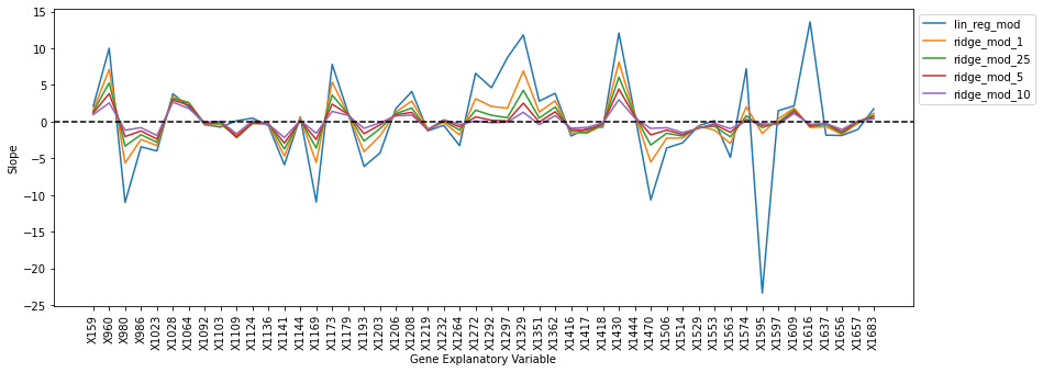
We might further inspect the ridge regression slopes by dividing each slope by it's original linear regression model slope to measure the factor by which it changed.
df_slopes_normalized = df_slopes.div(df_slopes['lin_reg_mod'], axis=0)
df_slopes_normalized| lin_reg_mod | ridge_mod_1 | ridge_mod_25 | ridge_mod_5 | ridge_mod_10 | |
|---|---|---|---|---|---|
| X159 | 1.0 | 0.747402 | 0.650437 | 0.562447 | 0.456821 |
| X960 | 1.0 | 0.711911 | 0.529032 | 0.382433 | 0.255760 |
| X980 | 1.0 | 0.511343 | 0.302736 | 0.183973 | 0.105341 |
| X986 | 1.0 | 0.707398 | 0.519205 | 0.370256 | 0.237502 |
| X1023 | 1.0 | 0.817974 | 0.705650 | 0.594866 | 0.472910 |
| X1028 | 1.0 | 0.880357 | 0.827802 | 0.777427 | 0.699601 |
| X1064 | 1.0 | 1.291372 | 1.280401 | 1.121231 | 0.893639 |
| X1092 | 1.0 | 1.009945 | 0.787079 | 0.515063 | 0.235389 |
| X1103 | 1.0 | 0.574198 | 0.219984 | 0.030592 | -0.043472 |
| X1109 | 1.0 | -14.970821 | -17.986539 | -16.907278 | -13.533319 |
| X1124 | 1.0 | -0.441828 | -0.521245 | -0.200419 | 0.262402 |
| X1136 | 1.0 | 0.643937 | 0.456077 | 0.465673 | 0.615949 |
| X1141 | 1.0 | 0.797689 | 0.634790 | 0.497879 | 0.367550 |
| X1144 | 1.0 | 0.822271 | 0.380908 | 0.228005 | 0.227921 |
| X1169 | 1.0 | 0.508491 | 0.328901 | 0.221682 | 0.143543 |
| X1173 | 1.0 | 0.691660 | 0.464884 | 0.305722 | 0.179910 |
| X1179 | 1.0 | 0.860198 | 0.860409 | 0.825274 | 0.703750 |
| X1193 | 1.0 | 0.671786 | 0.433470 | 0.269281 | 0.148944 |
| X1203 | 1.0 | 0.452781 | 0.221662 | 0.101905 | 0.034937 |
| X1206 | 1.0 | 0.739578 | 0.614248 | 0.528745 | 0.435154 |
| X1208 | 1.0 | 0.687672 | 0.450383 | 0.308540 | 0.218874 |
| X1219 | 1.0 | 0.788234 | 0.880653 | 0.923488 | 0.872686 |
| X1232 | 1.0 | 0.239174 | -0.144797 | -0.381228 | -0.539760 |
| X1264 | 1.0 | 0.556533 | 0.349586 | 0.219248 | 0.121859 |
| X1272 | 1.0 | 0.473943 | 0.237585 | 0.098102 | 0.014378 |
| X1292 | 1.0 | 0.450509 | 0.188569 | 0.043309 | -0.031000 |
| X1297 | 1.0 | 0.210792 | 0.062492 | 0.010019 | -0.008832 |
| X1329 | 1.0 | 0.585601 | 0.361993 | 0.213947 | 0.109041 |
| X1351 | 1.0 | 0.467729 | 0.176577 | -0.017598 | -0.145617 |
| X1362 | 1.0 | 0.737976 | 0.518372 | 0.350521 | 0.212010 |
| X1416 | 1.0 | 0.805035 | 0.647963 | 0.540778 | 0.455293 |
| X1417 | 1.0 | 1.709159 | 1.554903 | 1.242263 | 0.846682 |
| X1418 | 1.0 | 0.680785 | 0.506503 | 0.347428 | 0.206286 |
| X1430 | 1.0 | 0.673512 | 0.503303 | 0.369483 | 0.249546 |
| X1444 | 1.0 | 0.984324 | 0.866887 | 0.699458 | 0.500359 |
| X1470 | 1.0 | 0.516106 | 0.298442 | 0.168720 | 0.085630 |
| X1506 | 1.0 | 0.627155 | 0.439978 | 0.321287 | 0.231381 |
| X1514 | 1.0 | 0.776309 | 0.681384 | 0.605958 | 0.516626 |
| X1529 | 1.0 | 1.079816 | 1.386509 | 1.600980 | 1.617440 |
| X1553 | 1.0 | -9.013841 | -5.019273 | -3.101436 | -1.846966 |
| X1563 | 1.0 | 0.615063 | 0.427232 | 0.296659 | 0.196200 |
| X1574 | 1.0 | 0.279781 | 0.111315 | 0.042287 | 0.011108 |
| X1595 | 1.0 | 0.069013 | 0.035062 | 0.021207 | 0.012478 |
| X1597 | 1.0 | 0.257335 | -0.059367 | -0.204073 | -0.261971 |
| X1609 | 1.0 | 0.861574 | 0.754364 | 0.644358 | 0.519440 |
| X1616 | 1.0 | -0.057381 | -0.049934 | -0.037993 | -0.026131 |
| X1637 | 1.0 | 0.374506 | 0.203240 | 0.148317 | 0.138347 |
| X1656 | 1.0 | 0.919121 | 0.851737 | 0.724979 | 0.565422 |
| X1657 | 1.0 | 0.225496 | 0.013891 | -0.073043 | -0.089422 |
| X1683 | 1.0 | 0.642919 | 0.474178 | 0.351892 | 0.223972 |
We see that as the value of $\lambda$ is increased, there are some slopes (like X980) that dramatically decline in magnitude compared to their original magnitude in the linear regression model. On the other hand, there were other slopes (like X1109) that dramatically increased in magnitude compared to their original magnitude in the linear regression model.
plt.figure(figsize=(14,5))
plt.plot(df_slopes_normalized['ridge_mod_1'], label='ridge_mod_1')
plt.plot(df_slopes_normalized['ridge_mod_25'], label='ridge_mod_25')
plt.plot(df_slopes_normalized['ridge_mod_5'], label='ridge_mod_5')
plt.plot(df_slopes_normalized['ridge_mod_10'], label='ridge_mod_10')
plt.axhline(0, color='black', linestyle='--')
plt.ylabel('Percent of Linear Regression Slope')
plt.xlabel('Gene Explanatory Variable')
plt.xticks(rotation=90)
plt.ylim([-1,2])
plt.legend(bbox_to_anchor=(1,1))
plt.show()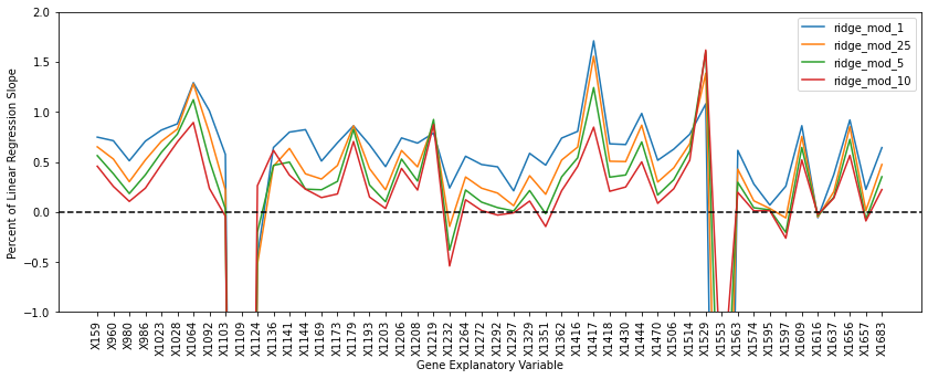
Which model is best?
Finally, let's determine which ridge regression model is best for the purpose of predicting the size of new breast tumors, by again comparing the test data R^2 of each model.
Given that one of our goals is to build a model that will yield good predictions for new breast tumors, let's inspect the test dataset R^2 of each of these 3 LASSO models.
Nonregularized Linear Regression Model: Test Dataset R^2
lin_reg_mod.score(X_test, y_test)-0.3071595344334954
Ridge Regression Model 1: $\lambda=1$ Test Dataset R^2
ridge_mod_1.score(X_test, y_test)0.12825147516877422
Ridge Regression Model 2: $\lambda=2.5$ Test Dataset R^2
ridge_mod_25.score(X_test, y_test)0.24810734542753
Ridge Regression Model 3: $\lambda=5$ Test Dataset R^2
ridge_mod_5.score(X_test, y_test)0.27410328541870965
Ridge Regression Model 4: $\lambda=10$ Test Dataset R^2
ridge_mod_10.score(X_test, y_test)0.2607143483417401
We can see that the linear ridge regression model that achieves the best test dataset R^2=0.274 is the model that used $\lambda=5$. Ideally, a more complete analysis would try out many other values of $\lambda$ to see if we can find a test dataset R^2 that was even higher. Notice, that this ridge regression model was not quite as high as the best LASSO model that we found with a test dataset R^2=0.279.
| Best Test R^2 | |
| Nonregularized Linear Regression | -0.307 |
| LASSO Linear Regression | 0.279 |
| Linear Ridge Regression | 0.274 |
Can we trust the non-zero slope interpretations in our chosen ridge regression model?
Ideally, we'd be able to trust our interpretations of our non-zero slopes in this resulting ridge regression model that we chose as well. Because ridge regression is more effective at downplaying the impacts of multicollinearity (which we know this dataset has), we may be able to trust the interpretive value of the slopes in our ridge regression more.
Notice how the magnitude of some slopes dramatically changed in the two models below.
df_slopes = pd.DataFrame({'lin_reg_mod': lin_reg_mod.coef_.T,
                         'ridge_mod_5': ridge_mod_5.coef_.T}, index=X_train.columns)
df_slopes| lin_reg_mod | ridge_mod_5 | |
|---|---|---|
| X159 | 2.093903 | 1.177710 |
| X960 | 9.995326 | 3.822538 |
| X980 | -10.996647 | -2.023085 |
| X986 | -3.413999 | -1.264054 |
| X1023 | -3.991874 | -2.374631 |
| X1028 | 3.797146 | 2.952002 |
| X1064 | 2.006906 | 2.250205 |
| X1092 | -0.408996 | -0.210659 |
| X1103 | -0.739345 | -0.022618 |
| X1109 | 0.121617 | -2.056208 |
| X1124 | 0.488547 | -0.097914 |
| X1136 | -0.547525 | -0.254968 |
| X1141 | -5.867328 | -2.921222 |
| X1144 | 0.657140 | 0.149831 |
| X1169 | -10.944499 | -2.426202 |
| X1173 | 7.801992 | 2.385242 |
| X1179 | 1.212503 | 1.000648 |
| X1193 | -6.094789 | -1.641212 |
| X1203 | -4.274063 | -0.435549 |
| X1206 | 1.790304 | 0.946614 |
| X1208 | 4.107494 | 1.267326 |
| X1219 | -1.244601 | -1.149374 |
| X1232 | -0.493502 | 0.188137 |
| X1264 | -3.258595 | -0.714440 |
| X1272 | 6.584962 | 0.646001 |
| X1292 | 4.623105 | 0.200222 |
| X1297 | 8.719397 | 0.087360 |
| X1329 | 11.802248 | 2.525056 |
| X1351 | 2.802728 | -0.049321 |
| X1362 | 3.868178 | 1.355878 |
| X1416 | -1.948134 | -1.053509 |
| X1417 | -0.923660 | -1.147429 |
| X1418 | -0.726373 | -0.252362 |
| X1430 | 12.056850 | 4.454804 |
| X1444 | 0.971105 | 0.679247 |
| X1470 | -10.656927 | -1.798032 |
| X1506 | -3.580033 | -1.150218 |
| X1514 | -2.879311 | -1.744741 |
| X1529 | -0.556923 | -0.891623 |
| X1553 | 0.126864 | -0.393462 |
| X1563 | -4.857389 | -1.440987 |
| X1574 | 7.214710 | 0.305086 |
| X1595 | -23.334004 | -0.494847 |
| X1597 | 1.487872 | -0.303635 |
| X1609 | 2.157559 | 1.390239 |
| X1616 | 13.586829 | -0.516199 |
| X1637 | -1.837732 | -0.272567 |
| X1656 | -1.881983 | -1.364397 |
| X1657 | -1.060942 | 0.077494 |
| X1683 | 1.749397 | 0.615599 |
Elastic Net Regression (ie. L1 and L2 Penalty Term)
We can see that this is a combination of the:
- L1 norm $\left[|\hat{\beta}_1|+|\hat{\beta}_2|+...+|\hat{\beta}_{50}|\right]$ from LASSO regression
- L2 norm $\left[\hat{\beta}_1^2+\hat{\beta}_2^2+...+\hat{\beta}_{50}^2\right]$ from ridge regression.
Similar to LASSO and ridge regression, we introduce a parameter $\lambda\geq 0$ that we must preselect. We also now use an $0\leq \alpha\leq 1$ parameter that we must also preselect.
The Ideal Scenario
Similar to the LASSO and ridge linear regression, the absolute best intercept and slope solutions to this optimization would be ones in which:
- $SSE=\left[ \sum_{i=1}^n(y_i-(\hat{\beta}_0+\hat{\beta}_1x_{i,1}+...+\hat{\beta}_{50}x_{i,50}))^2 \right]=0$
- $\lambda\cdot\left[\alpha\left[|\hat{\beta}_1|+|\hat{\beta}_2|+...+|\hat{\beta}_{50}|\right]+ \frac{1-\alpha}{2} \left[\hat{\beta}_1^2+\hat{\beta}_2^2+...+\hat{\beta}_{50}^2\right]\right]=0$
The Penalty Term Balancing Act
However, similarly, this "ideal scenario" that we just described is unrealistic. We also see that choosing intercepts and slopes that lead to a decrease of one term, often leads to an increase in the other term, and vice versa.
The Impact of $\lambda$
For similar reasons described when we used $\lambda$ in the LASSO linear regression, we see the following impact of $\lambda$ on our results.
$\lambda$ is Set Low
- $\lambda\cdot\left[\alpha\left[|\hat{\beta}_1|+|\hat{\beta}_2|+...+|\hat{\beta}_{50}|\right]+ \frac{1-\alpha}{2} \left[\hat{\beta}_1^2+\hat{\beta}_2^2+...+\hat{\beta}_{50}^2\right]\right]$ Is Higher
- SSE tends to be lower (ie. the fit is better)
$\lambda$ is Set High
- $\lambda\cdot\left[\alpha\left[|\hat{\beta}_1|+|\hat{\beta}_2|+...+|\hat{\beta}_{50}|\right]+ \frac{1-\alpha}{2} \left[\hat{\beta}_1^2+\hat{\beta}_2^2+...+\hat{\beta}_{50}^2\right]\right]$ Is Lower
- SSE tends to be higher (ie. the fit is worse)
Which slope magnitudes get to stay large?
Similar to LASSO and ridge regression, the resulting optimal slopes that are set "low", are the ones that bring the least predictive power to the model and thus are the most likely variable to overfit the model.
The Impact of the $\alpha$ Parameter
Now, let's explore the impact that $\alpha$ has on our resulting slopes.
-
$\alpha$ is Set High
When $\alpha$ is set higher, the penalty coefficient in front of the L1 term $\left[|\hat{\beta}_1|+|\hat{\beta}_2|+...+|\hat{\beta}_{50}|\right]$ becomes higher. Thus, the optimization problem is going to try harder to keep this term in particular low. Thus, your results slopes will tend to look more like those that were returned by LASSO regression (ie. zeroing slopes out). -
$\alpha$ is Set High
Alternativly, When $\alpha$ is set lower, the penalty coefficient in front of the L2 term $\left[\hat{\beta}_1^2+\hat{\beta}_2^2+...+\hat{\beta}_{50}^2\right]$ becomes higher. Thus, the optimization problem is going to try harder to keep this term in particular low. Thus, your results slopes will tend to look more like those that were returned by ridge regression (ie. less zeroing slopes out and more focus on balancing the weight in collinear slopes).
Less Clear Slope Interpretation Depending on $\alpha$
The smaller the value of $\alpha$ is set, ie. the more the returned slopes tend to resemble a ridge regression solution, the less the small slopes will be set exactly equal to 0. Thus, the less the slopes have interpretive value about which variables should be removed from the model because they do not bring enough predictive power.
Benefits of Elastic Net Regression
The benefits of elastic net regression is that it essentially can provide a "middle ground" solution between the type of results that you might get with LASSO and ridge regression. By toggling the $\alpha$ parameter, you can have your results resemble the type of solutions that you might get with LASSO vs. ridge regression to varying degrees.
Elastic Net Linear Regression for Predicting Tumor Size
Finally, let's actually apply our elastic netlinear regression model to this dataset.
Recall that our linear ridge regression objective function required for us to preselect a value for $\lambda$. Let's try out a series of different $\lambda$ values to see which model yields the best test dataset performance.
Also recall, that we need to preselect our $\alpha$ value as well. A more complete analysis would also try out many different combinations of $\alpha$ and $\lambda$ values to assess which model gave us the best test data results. However, for now we will just try $\alpha=0.7$. Because this $\alpha$ is higher and closer to 1, we might expect our resulting slopes to resemble more what we might get with a LASSO model.
We can similarly use the ElasticNet() function to fit a linear ridge regression model. This ElasticNet() function operates in a similar way to the Lasso() function. Let's be careful about the parameters here.
- the alpha parameter in the ElasticNet() function below represents the $\lambda$ parameter in the objective function above
- the l1_ratio parameter in the ElasticNet() function below represents the $\alpha$ parameter in the objective function above.
Fitting Four Elastic Net Linear Regression Models
Model 1: $\lambda=0.01$
from sklearn.linear_model import ElasticNet
en_mod_1 = ElasticNet(alpha=.01, l1_ratio=0.7)
en_mod_1.fit(X_train, y_train)
en_mod_1.score(X_test, y_test)
0.06547371156125181
Model 2: $\lambda=0.025$
en_mod_2 = ElasticNet(alpha=.025, l1_ratio=0.7)
en_mod_2.fit(X_train, y_train)
en_mod_2.score(X_test, y_test)
0.23638055648260659
Model 3: $\lambda=0.05$
en_mod_3 = ElasticNet(alpha=.05, l1_ratio=0.7)
en_mod_3.fit(X_train, y_train)
en_mod_3.score(X_test, y_test)
0.28513850610195246
Model 4: $\lambda=0.1$
en_mod_4 = ElasticNet(alpha=.1, l1_ratio=0.7)
en_mod_4.fit(X_train, y_train)
en_mod_4.score(X_test, y_test)
0.2639254089412595
We can see that the elastic net model that used $\lambda=0.05$ and $\alpha=0.7$ achieved the highest test dataset R^2=0.285. Also note that this is the highest breast tumor test dataset R^2 that we have achieved so far out of all explored models!
| Best Test R^2 | |
| Nonregularized Linear Regression | -0.307 |
| LASSO Linear Regression | 0.279 |
| Linear Ridge Regression | 0.274 |
| Elastic Net Regression | 0.285 |
Inspecting the Slopes
Next, let's inspect and compare the slopes of the models that we've created so far. Notice how we do see some zeroed out slopes in our results, regardless of what $\lambda$ value that we chose. This makes sense as our $\alpha$ was set larger, and therefore it's results will look more similar to what we would get with a LASSO model.
Also take note, just like we observed with the LASSO models, the higher the value of $\lambda$, the more slopes that were zeroed out.
df_slopes = pd.DataFrame({'lin_reg_mod': lin_reg_mod.coef_.T,
                         'en_mod_1': en_mod_1.coef_.T,
                         'en_mod_2': en_mod_2.coef_.T,
                         'en_mod_3': en_mod_3.coef_.T,
                         'en_mod_4': en_mod_4.coef_.T}, index=X_train.columns)
df_slopes| lin_reg_mod | en_mod_1 | en_mod_2 | en_mod_3 | en_mod_4 | |
|---|---|---|---|---|---|
| X159 | 2.093903 | 1.615975 | 1.358475 | 1.090770 | 0.746052 |
| X960 | 9.995326 | 8.060144 | 6.416783 | 4.691085 | 3.088208 |
| X980 | -10.996647 | -6.965351 | -4.424210 | -2.278063 | -0.790220 |
| X986 | -3.413999 | -2.768931 | -2.033785 | -1.337220 | -0.347230 |
| X1023 | -3.991874 | -3.436708 | -3.000938 | -2.449317 | -1.895899 |
| X1028 | 3.797146 | 3.408037 | 3.099803 | 2.878624 | 2.596566 |
| X1064 | 2.006906 | 2.342968 | 2.535539 | 2.235952 | 1.875274 |
| X1092 | -0.408996 | -0.397558 | -0.324774 | -0.185855 | -0.058357 |
| X1103 | -0.739345 | -0.455390 | -0.000000 | -0.000000 | 0.000000 |
| X1109 | 0.121617 | -1.150149 | -1.963366 | -2.365472 | -2.082780 |
| X1124 | 0.488547 | -0.000000 | -0.027279 | -0.000000 | 0.000000 |
| X1136 | -0.547525 | -0.444500 | -0.169867 | -0.000000 | -0.000000 |
| X1141 | -5.867328 | -5.154343 | -4.223917 | -3.427463 | -2.432639 |
| X1144 | 0.657140 | 0.561424 | 0.000000 | 0.000000 | 0.000000 |
| X1169 | -10.944499 | -6.676555 | -4.148376 | -2.577002 | -1.177291 |
| X1173 | 7.801992 | 6.206625 | 4.338025 | 2.735242 | 1.235253 |
| X1179 | 1.212503 | 0.968695 | 0.854449 | 0.736727 | 0.616764 |
| X1193 | -6.094789 | -4.775227 | -3.214174 | -1.639569 | -0.323363 |
| X1203 | -4.274063 | -2.400150 | -1.116151 | -0.137988 | -0.000000 |
| X1206 | 1.790304 | 1.392953 | 1.051212 | 0.816235 | 0.499708 |
| X1208 | 4.107494 | 3.316898 | 2.327103 | 1.280175 | 0.465704 |
| X1219 | -1.244601 | -0.911206 | -1.015590 | -1.178560 | -1.090303 |
| X1232 | -0.493502 | -0.138169 | 0.000000 | 0.021508 | 0.080950 |
| X1264 | -3.258595 | -2.242385 | -1.352558 | -0.714238 | -0.103740 |
| X1272 | 6.584962 | 3.741728 | 1.846926 | 0.287312 | -0.000000 |
| X1292 | 4.623105 | 2.029130 | 0.645845 | 0.000000 | -0.000000 |
| X1297 | 8.719397 | 2.840941 | 0.280463 | 0.000000 | 0.000000 |
| X1329 | 11.802248 | 8.548955 | 5.633816 | 3.022931 | 0.706893 |
| X1351 | 2.802728 | 1.701263 | 0.793606 | 0.000000 | -0.081493 |
| X1362 | 3.868178 | 3.190280 | 2.289450 | 1.506066 | 0.582151 |
| X1416 | -1.948134 | -1.697054 | -1.417397 | -1.054065 | -0.862737 |
| X1417 | -0.923660 | -1.350689 | -1.247298 | -0.855488 | -0.535160 |
| X1418 | -0.726373 | -0.470412 | -0.305559 | -0.031378 | -0.031960 |
| X1430 | 12.056850 | 9.097448 | 7.165911 | 5.381811 | 3.670749 |
| X1444 | 0.971105 | 0.933859 | 0.851519 | 0.579380 | 0.000000 |
| X1470 | -10.656927 | -7.013554 | -4.483356 | -2.694715 | -0.960104 |
| X1506 | -3.580033 | -2.234497 | -1.437787 | -0.749208 | -0.397086 |
| X1514 | -2.879311 | -2.371968 | -2.073026 | -1.878219 | -1.737383 |
| X1529 | -0.556923 | -0.524987 | -0.509621 | -0.670207 | -0.730044 |
| X1553 | 0.126864 | -0.952337 | -0.286741 | -0.199374 | -0.069218 |
| X1563 | -4.857389 | -3.388552 | -2.341469 | -1.586088 | -0.925848 |
| X1574 | 7.214710 | 1.894890 | 0.000000 | -0.000000 | -0.000000 |
| X1595 | -23.334004 | -2.439731 | -0.791844 | -0.426136 | -0.141519 |
| X1597 | 1.487872 | 0.648474 | 0.000000 | -0.213069 | -0.250520 |
| X1609 | 2.157559 | 1.953701 | 1.663401 | 1.253879 | 0.854298 |
| X1616 | 13.586829 | -0.048237 | -0.309621 | -0.442962 | -0.382420 |
| X1637 | -1.837732 | -0.930020 | -0.362243 | -0.000000 | -0.000000 |
| X1656 | -1.881983 | -1.835605 | -1.779952 | -1.448525 | -0.985379 |
| X1657 | -1.060942 | -0.306691 | -0.000000 | -0.000000 | -0.000000 |
| X1683 | 1.749397 | 1.299685 | 0.837095 | 0.398304 | 0.000000 |
Can we trust the non-zero slope interpretations in our chosen elastic net model?
Ideally, we'd be able to trust our interpretations of our non-zero slopes in this resulting elastic net model that we chose which also happened to have the best test R^2.
Because we set $\alpha$ to be high, this means that our results more closely resembled a LASSO model solution. Thus, we'd also want to inspect whether the remaining explanatory variables (ie. those with non-zero slopes) were collinear. Unfortunately, we do see that quite a few of these remaining explanatory variables are still collinear. Thus we should be more cautious about interpreting the slopes in this model.
nonzero_slope_genes = df_slopes[np.abs(df_slopes['en_mod_3'])>0.00001].index
X_train_remaining = X_train[nonzero_slope_genes]

sns.heatmap(X_train_remaining.corr(),vmin=-1, vmax=1, cmap='RdBu')
plt.show()
On the other hand if we had set our $\alpha$ to be lower, that would mean that our results would closely resemble a ridge regression model solution, which inherently tends to mitigate the selection of slopes with unreliable interpretations due to multicollinearity.
Conclusion and Potential Shortcomings
Goal Assessment
Goal 1: Best Predictions for New Breast Tumors
Thus, if our first and foremost goal was to select a model which we think would perform the best predicting new breast tumor sizes, then we would select our model that achieved the highest test data R^2=0.285. This was our elastic net model with $\lambda=0.05$ and $\alpha=0.7$. However, as we mentioned above we cannot quite trust our slopes interpretations due the extent to which the elastic net model did not assist in dealing with the multicollinearity.
Goal 2: More Trust in Slope Interpretations
However, if our goal was to achieve a model in which we'd be able to trust the interpretations of our slopes more (in the unfortunate presence of highly multicollinar explanatory variables), then we might consider selecting one of our ridge regression models. In addition, the test data R^2=0.274 of our best ridge regression model was not too much lower than that of our best final model.
Analysis Shortcomings
In our analysis above, we created a single training and test dataset by randomly splitting the dataset using a random state of 102.
Let's perform this same analysis again but using a different random state = 207 when making this split.
#Creating a new set of training and test datasets
df_train_other, df_test_other = train_test_split(df, test_size=0.1, random_state=207)
X_train_other = df_train_other.drop(['size'], axis=1)
X_test_other = df_test_other.drop(['size'], axis=1)
y_train_other=df_train_other['size']
y_test_other=df_test_other['size']
#Fitting the linear regression model
lin_reg_mod = LinearRegression()
lin_reg_mod.fit(X_train_other, y_train_other)
print('Linear Regression Test R^2:',lin_reg_mod.score(X_test_other, y_test_other))Linear Regression Test R^2: -0.2213718065663819
Unfortuately, we see that by just choosing a different random state to split up the training and test dataset our analysis shows us different results.
- All of our elastic net model test data R^2 values are negative, indicating that all of our elastic net trained models were poor fits for the test dataset.
- The best elastic net model in this case the one with $\lambda=.1, \alpha=0.7$, because it had the highest test data R^2. Notice how this is a different $\lambda$ parameter than what was chosen in our first analysis.
#Fitting 4 elastnic net models with the same parameters as before
en_mod = ElasticNet(alpha=.01, l1_ratio=0.7)
en_mod.fit(X_train_other, y_train_other)
print('Elastic Net - alpha=0.01 Test R^2:',en_mod.score(X_test_other, y_test_other))

en_mod = ElasticNet(alpha=.025, l1_ratio=0.7)
en_mod.fit(X_train_other, y_train_other)
print('Elastic Net - alpha=0.025 Test R^2:',en_mod.score(X_test_other, y_test_other))

en_mod = ElasticNet(alpha=.05, l1_ratio=0.7)
en_mod.fit(X_train_other, y_train_other)
print('Elastic Net - alpha=0.05 Test R^2:',en_mod.score(X_test_other, y_test_other))

en_mod = ElasticNet(alpha=.1, l1_ratio=0.7)
en_mod.fit(X_train_other, y_train_other)
print('Elastic Net - alpha=0.1 Test R^2:',en_mod.score(X_test_other, y_test_other))
Elastic Net - alpha=0.01 Test R^2: -0.14750397218825695
Elastic Net - alpha=0.025 Test R^2: -0.11125207416411964
Elastic Net - alpha=0.05 Test R^2: -0.0856548712042815
Elastic Net - alpha=0.1 Test R^2: -0.04788700566442472
This highlights the fact that the act of selecting a single training and test dataset based on a single random state and basing your model selection decisions off can have consequences. Doing so introduces an element of randomness to your model selections. Notice how we get two sets of different slopes, particularly in which different sets of slopes are set to 0.
Based on the differing results that we observed above, you should be more skeptical that your final selected elastic net model from 8.4 will indeed be the best when it comes to predicting new breast tumor sizes.
df_slopes = pd.DataFrame({'best_en_mod_old_rs': en_mod_3.coef_.T,
                         'best_en_mod_new_rs': en_mod.coef_.T}, index=X_train.columns)
df_slopes| best_en_mod_old_rs | best_en_mod_new_rs | |
|---|---|---|
| X159 | 1.090770 | 0.896141 |
| X960 | 4.691085 | 3.026627 |
| X980 | -2.278063 | -0.695596 |
| X986 | -1.337220 | -0.654839 |
| X1023 | -2.449317 | -1.772806 |
| X1028 | 2.878624 | 3.673288 |
| X1064 | 2.235952 | 2.793303 |
| X1092 | -0.185855 | 0.180124 |
| X1103 | -0.000000 | 0.079758 |
| X1109 | -2.365472 | -1.569070 |
| X1124 | -0.000000 | -0.845917 |
| X1136 | -0.000000 | -0.252004 |
| X1141 | -3.427463 | -2.542786 |
| X1144 | 0.000000 | -0.149432 |
| X1169 | -2.577002 | -0.711118 |
| X1173 | 2.735242 | 1.602873 |
| X1179 | 0.736727 | 0.231466 |
| X1193 | -1.639569 | -0.143467 |
| X1203 | -0.137988 | -0.003595 |
| X1206 | 0.816235 | 0.000000 |
| X1208 | 1.280175 | 0.469925 |
| X1219 | -1.178560 | -0.860819 |
| X1232 | 0.021508 | -0.000000 |
| X1264 | -0.714238 | -0.000000 |
| X1272 | 0.287312 | -0.000000 |
| X1292 | 0.000000 | 0.447804 |
| X1297 | 0.000000 | -0.698379 |
| X1329 | 3.022931 | 1.575060 |
| X1351 | 0.000000 | -0.411561 |
| X1362 | 1.506066 | 0.897085 |
| X1416 | -1.054065 | -0.224134 |
| X1417 | -0.855488 | -0.690652 |
| X1418 | -0.031378 | -0.000000 |
| X1430 | 5.381811 | 2.728960 |
| X1444 | 0.579380 | 0.588187 |
| X1470 | -2.694715 | -1.334511 |
| X1506 | -0.749208 | -0.641218 |
| X1514 | -1.878219 | -0.146984 |
| X1529 | -0.670207 | -0.210893 |
| X1553 | -0.199374 | -0.434005 |
| X1563 | -1.586088 | -0.447769 |
| X1574 | -0.000000 | -0.000000 |
| X1595 | -0.426136 | -0.000000 |
| X1597 | -0.213069 | 0.696042 |
| X1609 | 1.253879 | 1.034474 |
| X1616 | -0.442962 | -0.000000 |
| X1637 | -0.000000 | 0.000000 |
| X1656 | -1.448525 | -1.876078 |
| X1657 | -0.000000 | 0.863375 |
| X1683 | 0.398304 | -0.270280 |